The Fundamental Theorem of Algebra
2026-08-31 | 2026-10-11
Estimated Reading Time: 64 minutes
Prologue
It once fell to my lot to teach Mathematics to first-year students at an Australian university. It is often said that you truly learn only when you start to teach. And so it was in my case.
As I dug deeper into what numbers are and how many sets of numbers there are or could be, I realized that there was a vast chasm of ignorance in my knowledge. The terrain that lay beyond was not yet mapped out in my mind.
The more I attempted to know, the more forbidding was the safety net around the scaffolding of abstract algebra that politely said, “Workers Only. Keep Out”. To cross that net and venture to understand what lies beyond it is the burden of this blog.
Our journey starts with the enigmatic equation \(x^2 + 1 = 0\). It wends its way around concepts like sets, fields, vector spaces, arithmetic closure, algebraic closure, polynomial roots, winding numbers, algebraic structure, and the work of two mathematical greats: Gauss and Galois, of whom we will look only at the former in this blog.
There are many brief excursions into side alleys before we resume our main journey. They explain as much abstract algebra, or topology, or some other mathematics, as needed, to help the reader mentally retain the developing image of mathematics without letting it dissolve into the foam of incomprehension or dust of despair.
The centrepiece is the Fundamental Theorem of Algebra, which is usually glossed over with a passing reference, and often without even a plausibility argument. Because of the theorem’s importance, I strike a balance here between being too rigorous and too lax, so that there is sufficient tension to sustain student interest, and sufficient detail to ensure that the proof is persuasive.
This blog is written for high school and first year students of mathematics whose primary interest is in the application of what they learn. Many of the pre-requisites have been covered in my other blogs, and links to them are peppered all over this blog. But, in order to make the reading self-contained and focused, I have condensed and repeated much of that material here so that this story is gripping. Questions are asked, and later answered, to highlight the evolution of mathematics as a logical science.
Prior reading
In my blogs The Wonder That Is Pi, and The Two Most Important Numbers: Zero and One, I have introduced what I call the number menagerie. Different types of numbers were inducted into the art of reckoning or arithmetic, which later flowered into the science of quantity and symmetry called mathematics.1
I also strongly recommend the unfamiliar reader to also read my blog Expressions, Equations, and Formulae to get a firmer footing on what we will discuss subsequently.
The equation that started it all: \(x^2 + 1 = 0\)
The equation \[\begin{aligned} x^2 + 1 &= 0\\ x^2 &= -1 \end{aligned}\qquad{(1)}\] triggered the great change which led from the real numbers to the complex numbers.
And why did the change happen? Because Equation 1 asserts that the square of a number can be negative. But, there is no real number whose square is negative. Hence, a new type of number having this property needed to be invented. It was granted an identifying tag \(i\) to show that it was imaginary, not real! Simply put, \[i^2 = -1.\qquad{(2)}\]
We may now proceed to factorize Equation 1 so: \[\begin{aligned} x^2 + 1 &= 0\\ x^2 - (-1) &= 0\\ x^2 - (i^2) &= 0\\ x^2 - i^2 &= 0\\ (x - i)(x + i) &= 0\\ x &= \pm i. \end{aligned}\qquad{(3)}\]
But where does \(\pm i\) live? Let us catch our breath first, with some definitions, and then answer this question.
Sets, Fields, Vector Spaces, and Closure
We now take our first detour to define some basic terms:
A set is a collection of objects obeying some criterion. For our purposes, sets are collections of numbers.
A binary operation acts on two members in a set to generate a result. If the result is always in the set, we say that the set is closed under that operation.
There are four standard arithmetic operations, namely, \(+, -. \times, \div\).
A set that is closed under these operations—where order does not matter for addition or multiplication, and division by zero is excluded—is called a field.2 A number system capable of arithmetic is a field.
A vector space consists of two sets: a set of vectors and a scalar field—like the real numbers—used to multiply or scale those vectors.
The rational numbers, \(\mathbb{Q}\), and real numbers \(\mathbb{R}\) are fields. The natural numbers, \(\mathbb{N}\), and integers, \(\mathbb{Z}\) are not fields. A field is a behavioural template and need not consist only of numbers; it could be a collection of other mathematical objects that obey the rules of a field.
Vectors arise naturally in Physics. They are usually drawn on paper with two perpendicular coordinate axes. Vectors are shown as line segments with arrowheads: their lengths denote magnitude, and arrows direction. Vectors reside in vector spaces.
Every field can be regarded as a vector space over itself, but not every vector space is a field, since vector spaces do not generally have multiplication defined between vectors.
The familiar three-dimensional space we inhabit is denoted as \(\mathbb{R}^3 = \mathbb{R} \times \mathbb{R} \times \mathbb{R}\), which is a Cartesian triple product space, where every point in space is given a unique triplet of three real numbers, denoting its position from some chosen origin. This triplet behaves as a vector.
The irrationals
The “holes” in the number line left by the integers were filled by the rational numbers. The remaining holes, like the number \(\sqrt{2}\) were supposedly to be filled by the irrationals. The first on my list of questions was how are the irrationals defined? How many are there? Is there any way of defining them other than as in the binary not rational classification?
Dedekind’s schnitt or cut
These questions also troubled the mathematicians of the mid-1800s. How does one define an irrational number without recourse to geometry? If the whole numbers are all we confidently have—numbers we can touch and relate to—how can we define something like \(\sqrt{2}\) without a geometric detour as the diagonal of a unit square?
I have given one solution to this conundrum in my blog How Are Numbers Built?. But the continued fraction expansions of numbers like \(\sqrt{2}\) and \(e\) and \(\pi\) are not generalizable. And without a way for the general irrational number to be defined, how do we know how many irrationals there are, and what their values are?
Richard Dedekind pondered this question and came up with a solution that was partly geometric and partly set-theoretic.3 The interested reader may consult Dedekind’s original work in translation for the details [1].
Where will the number menagerie end?
Once the real line, composed of the rationals and irrationals, was deemed complete, there was still Equation 1 to proclaim the inadequacy of the reals.
The thought that ran in my head was, “If the complex numbers well and truly account for the roots of polynomials like \(x^2 + 1\), could there be some other type of polynomial that would require an even larger repertoire of numbers in order for its roots to be solved?”
If white sheep are purely real numbers, and black sheep are complex numbers with non-zero imaginary parts, could there be brown sheep, representing another type of number entirely, that might be needed to solve even more demanding polynomial equations? Would sheep of even more colours be needed to meet future challenges? This was the disquieting thought that ran in my mind as I prepared to teach mathematics to surveyors and engineers.
Whither goes \(i\)?
We have the rational and irrational numbers filling the real number line “without any gaps”. There is no room for another type of number on the real line.
Because the numbers \(\pm i\) cannot be accommodated within it, we need to extend \(\mathbb{R}\) to place it. But the imaginary numbers are immiscible with the real numbers. They do not dissolve one into another like salt in water. They are more like grains of sand in water—distinguishable parts of one whole. A means must be found to accommodate the imaginary as well as the real numbers, while each retains its separateness and its properties.
A two-dimensional vector has components in two orthgonal or perpendicular directions, aligned with the \(x\) and \(y\) axes. Vectors are denoted as \(a\mathbf{i} + b\mathbf{j}\) where \(a\) and \(b\) are real numbers and \(\mathbf{i}\) and \(\mathbf{j}\) the unit vectors in the \(x\) and \(y\) directions respectively. The vector is a single entity although its orthogonal components are twin.
Could we not likewise, christen a complex number as a sum of two numbers, one real and the other imaginary, functioning as a single unit?
A complex number may be written as \(a(1) + b(i) = a + bi\).4 Clearly, the real number \(1\) and the imaginary unit \(i\) function like the orthogonal unit vectors \(\mathbf{i}\) and \(\mathbf{j}\), spanning the two-dimensional plane. So, we may identify the set of complex numbers, \(\mathbb{C}\), with a two-dimensional vector space. And pictorially, that is exactly what an Argand diagram is.
The one-dimensional real numbers on the real line have expanded into the two-dimensional complex numbers on the complex plane.
The field of complex numbers ℂ
We are now at the threshold of the expansion of the real numbers, \(\mathbb{R}\), into the complex numbers, \(\mathbb{C}\). Both \(\mathbb{R}\) and \(\mathbb{C}\) are fields. The addition of the imaginary unit \(i\) might be seen as an ad hoc and opportunistic expansion of the real number field merely to accommodate solutions to \(x^2 + 1 = 0\). But there is a deeper and wider logic to this expansion.
The addition of \(i\) has extended the solution space of polynomials beyond \(\mathbb{R}\). And this extension was necessitated by the quadratic equation, Equation 1. Adding \(i\) to \(\mathbb{R}\) creates an algebraic extension of \(\mathbb{R}\). This means the entire complex plane, \(\mathbb{C}\), is simply an algebraic extension of \(\mathbb{R}\). What does this mean?
The real numbers can be built from a single number, namely \(1\), multiplied by some factor. So, \[\begin{aligned} 5 &= 5 \times 1\\ -6.3 &= -6.3 \times 1 \end{aligned}\] The number \(1\) is the basic building block for the real numbers—like a LEGO® brick from which objects may be built. Accordingly, the number \(1\) qualifies as a basis vector for the one-dimensional vector space of the real numbers \(\mathbb{R}\). The scalar multipliers are also supplied by \(\mathbb{R}\) and include any real number.
The mathematical notation describing how \(\mathbb{R}\) is extended to \(\mathbb{C}\) goes like this: \[[\mathbb{C}:\mathbb{R}] = 2\qquad{(4)}\] What does this mean? The complex numbers \(\mathbb{C}\) are built from the scalar multipliers drawn from the real numbers \(\mathbb{R}\). Exactly two bricks or basis vectors, \(1\) and \(i\), are needed to do this. The dimension of \(\mathbb{C}\) is therefore 2.
\([\mathbb{C}:\mathbb{R}] = 2\) is a concise shorthand for the blueprint used to construct the complex numbers from the real numbers. It is a single-line mathematical haiku.
To reiterate, the complex numbers in \(\mathbb{C}\) may be built as a linear combination of the two numbers, \(1\) and \(i\). The dimension of \(\mathbb{C}\) is two, and its scalar multipliers are drawn from \(\mathbb{R}\).
Can we multiply two complex numbers? Yes we can, as detailed in my blogs A Tetrad of Captivating Problems, and Demystifying Fractional Powers.
It is usual to specify a vector space over a (scalar) field where the scalar multipliers are supplied by the field and the vectors by the vector space. We may say that \(\mathbb{C}\) is a vector space over the field \(\mathbb{R}\). Equally, we may say that \(\mathbb{C}\) is a vector space over the field \(\mathbb{C}\). Therefore, \(\mathbb{C}\) is both a field and a vector space.
The definitive discovery of Gauss
Once the real number line had been completed with a definition of the irrationals, the next examination of “vacancies” belonged in the realm of the complex numbers. Fortunately, Carl Friedrich Gauss banished the thought of numbers “above” the complex to solve complex polynomial equations with his Fundamental Theorem of Algebra, the subject of this blog.5 All we have are white and black sheep; we do not have sheep of other colours.
In this blog, the steps to the FTA are revealed in slow motion so as not to discourage the eager student who is just learning the ropes of algebra beyond the high school. Join this exciting journey!
Polynomials
In a previous blog, I have classified polynomials in the section entitled “the …nomial” family. Take a look at it if interested. For those needing a comprehensive refresher on polynomials, I highly recommend the student-friendly, free online textbook from OpenStax [2].
The polynomial originally arose from the study of algebra in which the solution of equations was the primary goal. Any arithmetic equation, however complicated it might look, can finally be reduced to a polynomial on the left side and zero on the right [3].6
Polynomials are continuous functions. If you graph a continuous function on paper, as the independent variable increases in value, you can trace the associated curve without lifting the pencil off the paper. This intuitive explanation of continuity is sufficient for our purpose in this blog.
When calculus evolved, polynomials were identified as continuous and differentiable functions with certain maxima-minima properties. Still later, it has been suggested that polynomials may be viewed as “… a clothesline on which we hang up a sequence of numbers for display.” [4]. If you are interested in polynomials and their place in the history of mathematics, Merzbach and Boyer is a good reference [5].
A real-valued function \(p\) assigns to each real input value \(x\) some real output value \(y\) according to some rule. This may be written as: \[\begin{aligned} p &: \mathbb{R} \to \mathbb{R}\\ p &: x \mapsto y\\ p(x) &= y \end{aligned}\qquad{(5)}\]
A polynomial is a continuous function [2] that has the specific form: \[p(x) = a_nx^n + a_{n - 1}x^{n - 1} + \dots + a_{1}x + a_0.\qquad{(6)}\]
If all the \(a_{i}\)’s are real numbers and \(n\) is not zero, we call this a real-valued polynomial of degree \(n\).
The definition of a polynomial is fixed by its equation, but the domain of its definition can be varied.
Plotting a real-valued polynomial
For \(p: \mathbb{R} \to \mathbb{R}\), the input variable, \(x \in \mathbb{R}\) is a real number. And so is the output variable \(p(x) = y \in \mathbb{R}\).
The familiar Cartesian plane, \(\mathbb{R}^2\), is actually two real number lines at right angles to each other. This setup is referred to as the Cartesian product of \(\mathbb{R}\) with itself, denoted by \(\mathbb{R}^2 = \mathbb{R} \times \mathbb{R}\). It leads to ordered pairs of real numbers \((x, y)\), which relate the output \(y\) to the input \(x\).
Let \(p\) be a real-valued polynomial. The roots of the polynomial are the values of the input that lead to zero output. If \(\alpha\) is a root, then, \(p(\alpha) = 0\).
Because the word “root” baffles some students, I will make a short detour to explain it here.
How did the word “root” arise?
There is a mystery behind the term “root” as applied to polynomials. Plants have roots. But why do polynomials have roots? It is because the Indian mathematicians used the word mūla (मूल) or root for what we call the root of a polynomial. And the Arab mathematicians faithfully translated mūla to jazr which also carries the sense of a plant root, or base, or foundation. The European mathematicians likewise translated jazr to radix or root.
These early mathematicians realized that the entire polynomial may be constructed from its roots—its base or foundation. Suppose I told you to construct a real polynomial with roots \(2\) and \(-3\). How would you go about it?
The value of a polynomial is zero when evaluated at its roots. And zero multiplied by any number, including zero, is zero. Therefore, if I multiplied the two linear factors \((x - 2)\) and \((x - (-3)) = (x + 3)\)—each of which evaluates to zero at the roots—I would get \[\begin{aligned} p(x) = y &= (x - 2)( x + 3)\\ &= x^2 + 3x -2x - 6\\ &= x^2 + x - 6 \end{aligned}\qquad{(7)}\] We can check this by substituting \(x = 2\) in Equation 7, to get \(4 + 2 - 6 = 6 - 6 = 0\). Likewise, if \(x = -3\), we get \(9 - 3 - 6 = 9 - 9 = 0\).
The roots of a plant are foundational to the plant, which grows from it. Likewise, we may construct the entire polynomial from its roots.
Roots and zero-crossings
Pictorially, when we plot a real polynomial—with \(x\)- and \(y\)-axes—in accordance with Equation 5, the roots are located at the points where the graph intersects or cuts the \(x\)-axis. The \(x\)-axis is also the line \(y = 0\).
The root(s) are those input values for which the output is zero.
Why is this important? Because roots force our attention to those inputs that yield a zero output. They succinctly relate a foundational aspect of the input-output relationship.
That is the true meaning of zero crossings in the context of finding the roots of real polynomials. The zeros being crossed are those of \(y\), not \(x\).7
Graph of \(p(x) = x^2 + 1\)
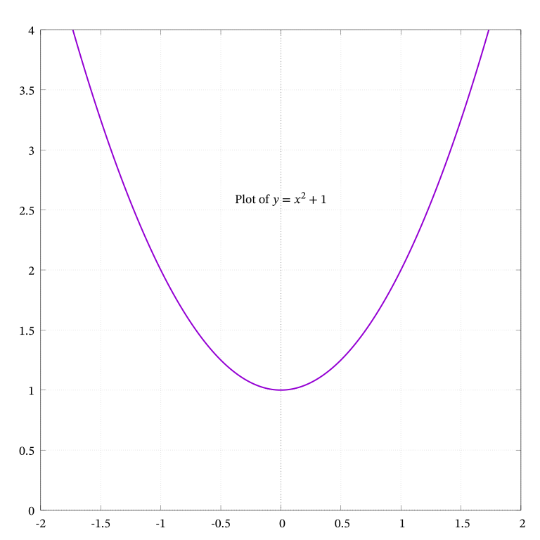
Consider the famous polynomial \(p(x) = x^2 + 1\) which has led us here. If we plot \(p(x) = y = x^2 + 1\) on \(\mathbb{R}^2\), we get Figure 1. The curve is a conic section called a parabola, which never crosses the \(x\)-axis. This means that the equation has no real solutions.
Before we look at the complex-valued version of the same polynomial, we need to look at a theorem that constrains continuous functions to behave in a certain way.
The Intermediate Value Theorem (IVT)
When a real polynomial is plotted on co-ordinate axes, the input ranges from the very negative to the very positive. We have to carefully track the zero-crossings to determine the roots.8
Before plotting the same polynomial with two different domains, I want to make a small detour into something called the Intermediate Value Theorem.
The essence of the Intermediate Value Theorem (IVT) is:
“If you are an ant crawling on a table, you cannot cross a line without touching it.”
In mathematical terms, if a function \(p: \mathbb{R} \to \mathbb{R}\) is continuous within an interval \([a, b]\), then for any value \(u\) between \(p(a)\) and \(p(b)\), there exists some \(c \in (a, b)\) for which \(p(c) = u\).
Consequently, if \(p(a)\) and \(p(b)\) are opposite in sign, there must exist some \(c \in (a, b)\) for which \(p(c) = 0\). This is called the Theorem of (Bernard) Bolzano.
In other words, a continuous function, like a polynomial, that changes sign within a closed interval must assume the value zero at some point inside that interval. A corollary of this theorem is that all real, odd-degree polynomials must have at least one real root.
Redefining the domain
We have seen that if we re-define the function \(p\) to have a complex domain, solutions do exist for \(p(x) = x^2 + 1 = 0\).
Let us now define a complex-valued polynomial \(P\) so: \[\begin{aligned} P &: \mathbb{C} \to \mathbb{C}\\ P &: z \mapsto w\\ P(z) &= w\\ z &= x + iy\\ w &= u + iv. \end{aligned}\qquad{(8)}\]
Specifically, let the definition of \(P\) mirror that of \(p\): \[P(z) = z^2 + 1.\qquad{(9)}\]
Observe the change in notation. The lowercase \(p\) for the real function has become the uppercase \(P\) for the complex function. The real variable \(x\) has become the complex ordered pair \(z\). The real output \(y\) has become the complex output \(w\).9 It must emphasized that the polynomial is the same, only its domain has been re-defined.
Through this redefinition, we have gained a solution where there was none previously. Categorically, \(P(z) = z^2 + 1 = 0\) implies \(z = \pm i\). Let us now explore how this happens.
Gauss and his proof
The Fundamental Theorem of Algebra (FTA) states that every non-constant polynomial of a single variable, with complex coefficients, must have at least one complex root. Here complex root also includes real roots.
This statement is also equivalent to saying that every non-constant polynomial, \(P(z)\), of degree \(n\) with complex coefficients, has exactly \(n\) complex roots, where repeated roots are counted as separate roots.
Gauss presented a proof in 1799 that relied on a geometric intuition that we will look at carefully in this blog. But because they could find gaps in the logic where Gauss had made a leap of the imagination, not all mathematicians agreed with his proof.
The branch of mathematics called topology that deals with spatial properties had not been invented at the time Gauss presented his proof. It was only after Alexander Ostrowski filled the gap in 1920, that the mathematical community accepted the first proof of Gauss on the FTA.
This theorem allows mathematicians to heave a sigh of relief that no more unusual types of numbers are lying in wait to pounce upon them at an opportune moment in the future. It also puts paid to my concern about brown sheep, and sheep of other colours.
But how is this grand reassurance earned? A good start would be to extend the IVT to two dimensions and see a visual demonstration of the theorem.
Gauss did not use complex polynomials at the time he presented his proof. But the substance of what he did was to adapt the IVT to the case of a complex polynomial. We will follow the steps that were taken through then uncharted mathematical territory to tame the roots of complex polynomials.
The complex polynomial \(P(z) = z^2 + 1\)
Let us define our complex polynomial so: \[\begin{aligned} P &: \mathbb{C} \to \mathbb{C}\\ P &: z \mapsto z^2 + 1\\ P(z) &= z^2 + 1 = w. \end{aligned}\qquad{(10)}\]
\(P\) takes a complex value, \(z\), as input and maps it to another complex value, \(P(z) = z^2 + 1 = w\), as output.
Recall that the input real line for a real polynomial is designated \(x\) and is different from the output real line, which is designated \(y\).
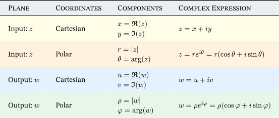
Likewise, for complex-valued functions, the input complex plane is designated \(z\) and the output complex plane is designated \(w\). In fact, this is written out in full as: \[\begin{aligned} z &= x + iy\\ w &= u + iv. \end{aligned}\qquad{(11)}\] Not keeping this distinction clearly in mind can cause grief later on. So, it is worthwhile taking some time to anchor in these key concepts right at the beginning. For a start, take a piece of paper and draw the input and output complex planes separately and label their axes. Draw a line with an arrowhead showing the path from input to output.
The complex zero, is defined as \((0, 0)\): its real and imaginary parts are both equal to zero. For convenience, we write it simply as \(0\).
The roots of a complex polynomial occur when the graph of the complex polynomial passes through the point \((0, 0)\). Symbolically, if \(z_{0}\) is a root of \(P\), \(P(z_{0}) = 0\).
How do we plot complex functions?
As noted previously, the input as well as the output of a complex polynomial is a two-dimensional vector. So, how do we plot a complex polynomial on a two-dimensional plane? Clearly, something must give. But what is it that gives?
We trade in our ability to see a graphical picture of the entire function at once, as in Figure 1. We must view it in parts or instalments. Let us see how to accomplish this.
A real-valued function of a real variable fits neatly into the two-dimensional graphical representation \(\mathbb{R}^2\) of Figure 1.
Since a complex number has two parts, graphing a complex-valued function of a complex variable means that we have to contend with a total of four variables: two input and two output. But we do not encounter four axes in our daily experience!
How do we accommodate complex polynomials into the two-dimensional plane? This dilemma was faced by mathematicians in the early days of complex function plotting.
If this question has never occurred to you, kindly pause awhile to ponder it. By asking such fundamental questions, you deepen your understanding of the subject, and also attune your thinking to how it evolved.
Injecting rigour into the notation
With two complex planes and four variables, there is ample scope for confusion and ambiguity when dealing with complex polynomials. Let us settle the notation unequivocally first. We enumerate the following:
Let the polynomial \(P\), of degree \(n \geq 1\), with real coefficients, map one complex number to another.
Let the output of \(P\) be single-valued rather than multi-valued.
Let the input complex plane be called the \(z\)-plane with \(z = x + iy\).
Let the output complex plane be called the \(w\)-plane with \(w = u + iv\).
Let the third vertical axis, if used, be called the \(\zeta\)-axis, or zeta axis, to avoid confusion with the input variable \(z\).
Then, \(P(x + iy) = P(z) = w = u + iv\).
We may now write down the following mathematical statements to avoid confusion about what is being referred to at any stage of the visualization of the complex polynomial. \[\begin{aligned} P &: \mathbb{C} \to \mathbb{C}\\ P &: z \mapsto P(z)\\ P &: z \mapsto w\\ P &: (x + iy) \mapsto (u + iv)\\ P(z) &= a_nz^n + a_{n-1}z^{n-1} + \dots + a_1z + a_0 \text{, with $n \in \mathbb{Z}$ ; $n \geq 1$ and $a_i \in \mathbb{R}$}\\ P(z) &= P(x + iy)\\ &= w\\ &= u + iv\\ \end{aligned}\qquad{(12)}\]
For the polar parametrization, we may write: \[\begin{aligned} z &= r e^{i\theta}\\ w &= \rho e^i{\varphi}\\ P(z) &= P(r e^{i\theta})\\ &= \rho e^{i\varphi}\\ &= w \end{aligned}\qquad{(13)}\]
As you can see, it is quite a mouthful, but we will not get into strife if we keep the variables dis-entangled as we go along.
Plotting complex functions to visualize them
Plotting complex functions is like trying to stuff too many things into a small suitcase. Something has to give. For example, instead of taking an extra pair of shoes, you might take just the pair you are wearing and save some space. The critical question is “What gives?”.
The book by Needham entitled Visual Complex Analysis [6] will prove invaluable for visualizing complex functions. Do refer to it if you get stuck or are confused.10
Physicists and engineers need to plot complex functions as part of their work. It is therefore a subject, not only of academic, but also practical importance.
Because I do not find it easy to visualize complex function plots, I will be taking detours to anchor in key concepts, and explain what happens in slow motion. Please bear with me.
Mapping the \(z\) and \(w\)-planes side by side
If there is a definitive, real McCoy representation of how a complex function is plotted showing both domain and co-domain, this is it. Taking the bull by the horns, we concede that four variables need two planes.
Traditionally, the input plane is called the \(z\)-plane, and its axes are the real and imaginary components of the input variables: \(z = x + iy\).
Likewise, the output plane is called the \(w\)-plane, and the real and imaginary parts of the output variables are called \(u\) and \(v\), i.e., \(w = u + iv\).
We plot the input on the \(z\)-plane on one side and the output on the \(w\)-plane on the other. Needless to say, the labels must clearly identify which plane we are looking at. Colours, arrows, or other devices may be used to match corresponding sets of inputs and outputs. But it does require the willingness and effort to visualize.
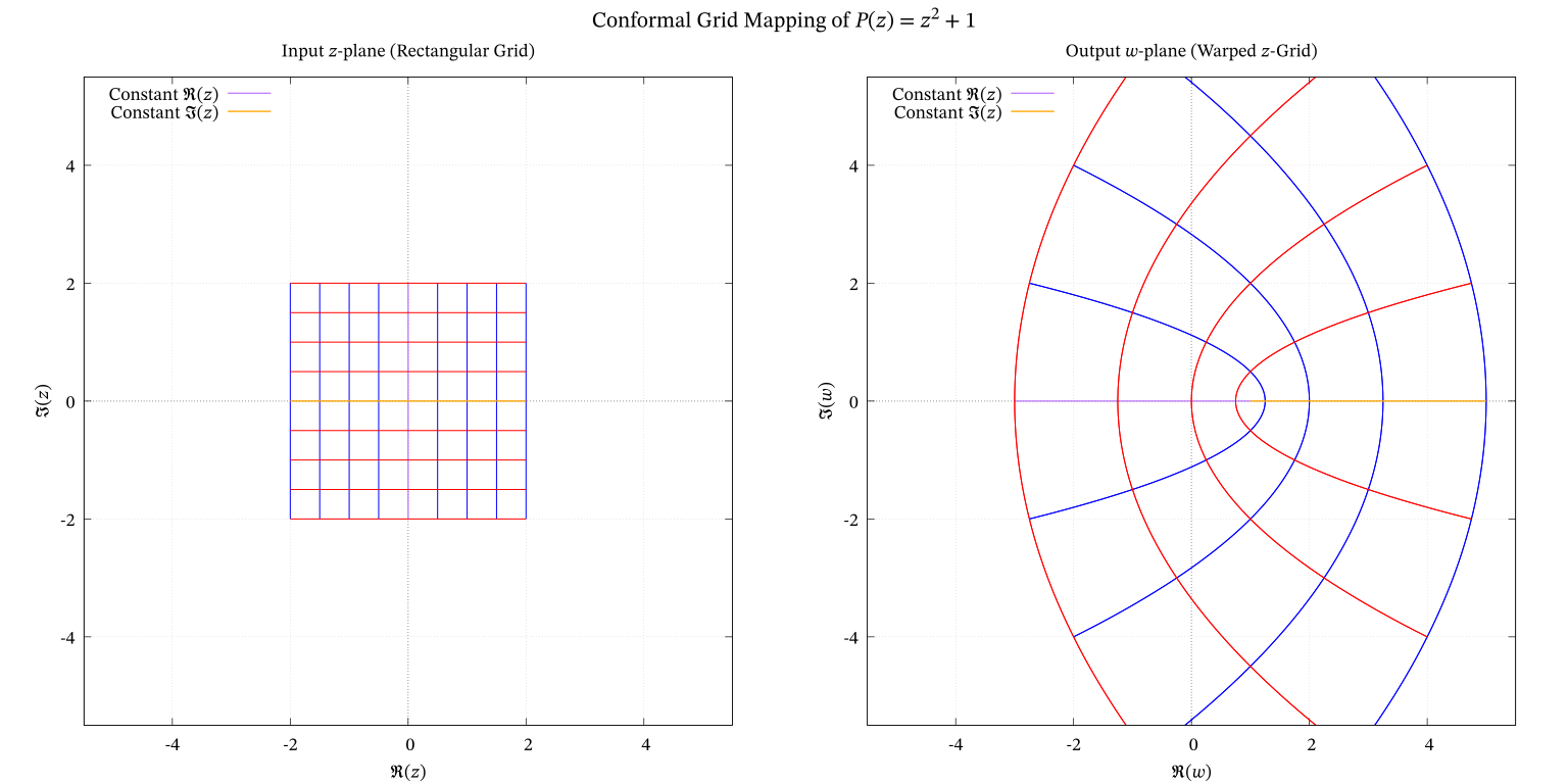
On the left, we have the rectangular grid of the input \(z\)-plane. On the right, we have the rectangular grid of the output \(w\)-plane. Then imagine that we feed the entire grid of values on the \(z\)-plane as inputs to the polynomial \(P(z)\), and that we plot the resulting outputs on the rectangular \(w\)-plane.
When \(P\) is continuous and differentiable, this process is called conformal mapping [6]. Lines that are orthogonal on the input plane retain their orthogonality on the output plane. Conformal mapping is an angle-preserving transformation.
For the case of \(P(z) = z^2 + 1\), we will have two graphs side-by-side. On the left, the undisturbed rectangular co-ordinate grid of the \(z\)-plane. On the right the values of \(P(z)\) plotted on the pristine \(w\)-plane.
Note that both planes are just that: two-dimensional planes. There is no vertical axis on either: so, no extraneous variable to confuse the issue. Figure 2 illustrates this.
There are several noteworthy points about the above two graphs:
Both graphs depict the complex plane. The one on the left shows the input \(z\)-plane, while the one on the right shows the output \(w\)-plane.
The origin at \((0, 0)\) on the \(z\)-plane has been mapped to \((1, 0)\) on the \(w\)-plane.
The red-and-blue lines on the rectangular grid on the left show the input. The red-and-blue lines on the right show the output.
The red-and-blue rectangular grid on the left has been warped by the polynomial \(P(z)\) into the red-and-blue parabolic grid superimposed on the \(w\)-plane. This is the clearest depiction of the action of the polynomial.
Although both the left and right images are on the same scale, the right image appears magnified in comparison to the original grid on the \(z\)-plane. This is due to squaring in the polynomial map.
The intersections of the lines in the transformed red-and-blue grid on the right are at ninety degrees just as in the original on the LHS.11 This feature of conformal mapping makes it valuable for solving practical problems.
Though they are fascinating, we do not need conformal mapping to prove the FTA, and so will now go on to other methods for plotting complex curves.
The Modulus Surface Plot and Cassini Contours
What can we do to reduce the plotting real estate and still get a good picture of what is going on? One solution is to use the third axis—the vertical axis on the \(z\)-plane, mutually perpendicular to the other two—and use it to represent some real-valued function of the output.
This hybrid setup, with the input variables on the base, complex plane and a real-valued function of the output on the vertical axis, allows us to better visualize some of the relationships we are trying to understand.
Let us use Equation 12 to re-orient ourselves to the variables: \[\begin{aligned} P(x + iy) &= P(z)\\ &= w\\ &= u + iv. \end{aligned}\] The absolute value, or magnitude, or modulus of a complex number, is a non-negative, real-valued function of the complex number. In our case, the modulus of \(P(z)\) is denoted and defined as: \[\begin{aligned} \lvert P(z) \rvert &= \lvert w \rvert\\ &= \sqrt{u^2 + v^2}. \end{aligned}\qquad{(14)}\] We may then collapse the output complex number \(P(z) = w\), with its two dimensions, to its one-dimensional modulus. This latter, being real and non-negative, may be easily represented on a single axis.
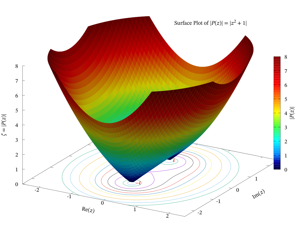
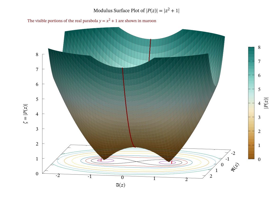
Thus, we could plot the input variables \(\Re(z)\) on the \(x\)-axis, \(\Im(z)\) on the \(y\)-axis, and the modulus of the output, \(\lvert P(z) \rvert\), on the vertical axis.12 We will call this third, vertical axis the \(\zeta\) axis to avoid confusion with \(z\).13 The resulting surface is called the modulus surface. It is a topographic representation of the absolute value of the output complex number mapped over the plane of the input complex number.
The modular surface of the complex polynomial \(P(z) = z^2 + 1\) is shown in Figure 3. Yet another view of the same surface is shown in Figure 4.
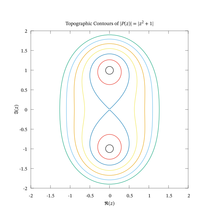
Observe from Figures 3,4 the following:
The complex plane at the base of both figures is the input complex plane or \(z\)-plane.
To avoid confusion with the \(z\)-plane, the vertical axis perpendicular to the base plane is called the \(\zeta\)-axis.
The modulus surface touches the base plane at only two points: the roots \(\pm i\).
The real parabola \(y = x^2 + 1\) is plotted and appears on the modulus surface, as shown in Figure 4. It does not ever contact the complex plane or the line \(y = 0\). This shows the consistency between the real-valued and complex-valued versions of the same equation.
The closed loops at the bottom of both figures are the topographic contour maps of the modulus surfaces. In our case, they are called Cassini ovals, and are illustrated in Figure 5.
The loci of fixed input circles
We have seen the transformation of a rectangular grid into a parabolic grid with conformal mapping. We have also seen the mapping of the modulus surface over the input complex plane to demonstrate the values of the complex roots, and appreciate why there are no real roots for \(P(z) = z^2 + 1 = 0\). But we have not seen any plots where the base plane is the output complex plane, and where the plots show something else. We examine that option here.14
Moreover, while the rectangular grid is transformed in conformal mapping, we have not seen how circles are transformed under the mapping of a polynomial. This is what we look at here.
We could use polar coordinates, specifically applied to complex numbers, to find a way out of the complex-to-complex plotting logjam. The two equivalent forms of representing a complex number are the Cartesian and polar forms. As noted in a previous blog: \[\begin{aligned} z &= x + iy\\ &= re^{i\theta}\\ &= r(\cos\theta + i\sin\theta)\\ \theta &= \arg(z) = \arctan\left({\frac{y}{x}}\right)\\ r &= \lvert z \rvert = \sqrt{x^2 + y^2} \end{aligned}\qquad{(15)}\] I will refer collectively to these equations as Equation 15.15
Since it is the set \(\mathbb{C}\) that yields the hard won solutions to the equation \(z^2 + 1 = 0\), we must somehow plot the curve on the complex plane to gain further insights.
The Cartesian to polar parameterization of Equation 15 holds one key to manageable graphing of complex functions without losing track of what is happening. We could keep some aspect of the input fixed and see how the output varies. This is a compromise solution.
We need to condense the input and link it somehow to the output. One way is to fix the input in some way and plot the output. Repeating this with several different inputs will give us a series of output curves. This is called parametriztion and is a well known device for parsimonious visualization.
The oft-adopted solution is to keep the modulus or absolute value,16 \(\lvert z \rvert = r\), of the input complex number fixed and plot the graph of the output on the complex plane. This is what we do below.
This method of plotting has various names. The two I prefer are image loop or argument vector trajectory. The former states that the curve is the image under the polynomial and the second that it tracks the path as input \(\theta\) is varied while \(r\) is kept constant. The first is succinct while the latter is more descriptive. I will mostly use image loop for brevity.
An image loop is the closed curve in the complex plane defined as the image of a circle under a complex polynomial mapping.
The complex number \(z\), expressed in polar form is \(z = re^{i\theta}\). The polar form of the polynomial \(P\) then is:17 \[\begin{aligned} P(z) &= (re^{i\theta})^2 + 1\\ &= r^2e^{i(2\theta)} + 1\\ &= r^2(\cos2\theta + i\sin2\theta) + 1\\ &= r^2(\cos2\theta) + i(r^2\sin2\theta) + 1\\ &= \rho\cos\varphi + i\rho\sin\varphi + 1\\ &= \rho e^{i\varphi} + 1. \end{aligned}\qquad{(16)}\] What does Equation 16 tell us? First: \[\begin{aligned} \rho &= r^2\\ \varphi &= 2\theta. \end{aligned}\qquad{(17)}\]
In addition, an input circle of radius centred on \((0, 0)\) on the input plane maps to an output circle of radius \(\rho\) whose center has been shifted by one unit to the right—to \((1, 0)\)—on the output real axis.
Because \(\varphi = 2\theta\), Equation 16 also tells us that the output “rotates” at twice the frequency of the input. When \(\theta\) moves one full circle on the input plane, the output has rotated twice on the output plane. The number \(2\) arises from the squared term \(z^2\). I will return to this point later in this blog, as it is key to understanding Gauss’s proof of the FTA.
What is the complex plane on which are plotting? Is it \(z\) or is it \(w\)? If you are confused, pause a while and think deeply. It will internalize your knowledge.
The complex polynomial, \(P\), is doing the mapping from \(z\) to \(w\). What is the input to the polynomial? Circles of constant \(r\) on the input \(z\)-plane. So the path is being traced on the output \(w\)-plane, which is the base complex plane. To keep the variables unambiguously separate, and as a mnemonic, use Figure 6:
We keep \(r\) fixed for a series of values, say, between \(1\) and \(10\), and for each case, we are plot the locus traced out by the polynomial on the \(w\)-plane. These curves may be distinguished by color or their line-type, and may be indexed to their respective values of \(r\).
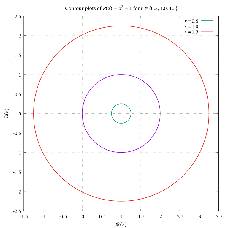
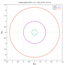
The parametric plot put out by gnuplot18 is shown in Figure 7. As stated above, the observant among you will notice that we have three concentric circles, all of whose centres have been shifted to the right of the origin by one unit.
The following observations are pertinent:
The contours of constant input \(r\) are obviously closed concentric circles on the \(z\)-plane.
Those contours of constant input \(r\) map to values of constant output \(\rho\) on the \(w\)-plane, which are also closed concentric circles.
The radii \(r\) and \(\rho\) are related by \(\rho = r^2\).
Although they are not shown, the input circles are centred at \((0, 0)\) on the \(z\)-plane.
The output circles are offset from the origin and are centred at \((1, 0)\) on the \(w\)-plane.
Because, \(\varphi = 2\theta\), for every increase of \(2\pi\) in the input argument \(\theta\), the output argument \(\varphi\) in the output curve cycles twice.
In Figures 3,4 the roots may be seen on the \(z\)-plane because the \(\zeta\)-axis also starts from zero on that plane.
But we cannot view the roots on the \(w\)-plane in Figure 7 because the input plane is not shown in it.
The roots of a complex polynomial are those values on the input plane which map to the origin \((0, 0)\) on the output plane.
We get the different contours by allowing \(r \geq 0\) to increase freely and trace out the paths dictated by \(\theta\) as it does so. Each value of \(r\) gives rise to a different coloured curve in Figure 7. By virtue of how \(P(z)\) is defined, the output curves in Figure 7 are circles, but thy need not always be so.
Contours of constant \(r\) are closed on the \(w\)-plane
Let \(P(z) = P(re^{i\theta})\) be an arbitrary complex polynomial of degree \(n \geq 1\). We can plot it by keeping the modulus \(r\) fixed and letting the argument \(\theta\) vary. We could then repeat the process by changing the fixed value of \(r\) and letting \(\theta\) vary again. The result would be a series of output contours generated by different fixed values of \(r\), as demonstrated by Figure 7.
How does such a plot behave? Since the trigonometric functions are periodic, we expect the plot on the output \(w\)-plane to close upon itself. Consider adding one revolution of \(2\pi\) to any arbitrary argument \(\theta\): \[\begin{aligned} P(re^{i(\theta + 2\pi)}) &= P(re^{i\theta}e^{i2\pi}); \text{ since $e^{i2\pi} = 1$,}\\ &= P(re^{i\theta}(1))\\ &= P(re^{i\theta}) \end{aligned}\]
The complex polynomial curve of \(P(z) = P(re^{i\theta})\) is closed for each value of \(\lvert z \vert = r\).
Why only three curves?
Why plot only three curves in Figure 7? That is an astute question. These three curves were chosen as snapshots—out of an uncountable infinity of curves—because they serve as examples of three different behaviours:
The \(r = 0.5\) case shows that the output circle has a radius \(\rho\) smaller than \(r\) since \(\rho = r^2 = 0.25 < r = 0.5\) when \(r < 1\). Circles whose input radius \(r < 1\) have output radii \(\rho < 1\) and therefore cannot pass through the origin \((0, 0)\) because the circles are centred on \((u, v) = (1, 0)\). The solution space for the roots excludes circles with radii \(\rho < 1\), and consequently with \(r < 1\).19
When \(r = 1\), we have the input and output circles equal in radius. But this is not the only reason for choosing this \(r\) value. The output circle is tangent to the line \(u = 0\) which is the imaginary axis of the \(w\)-plane.
The circle first passes through \((0, 0)\) when \(\varphi = \pi\), which means \(\theta = \frac{\pi}{2}\). The root on the input plane is \((r\cos\frac{\pi}{2}, ir\sin\frac{\pi}{2}) = (\cos\frac{\pi}{2}, i\sin\frac{\pi}{2}) = (0, i)\).
The other occasion when the output locus touches \((0, 0)\) is when \(\varphi = 3\pi\) which corresponds to \(\theta = \frac{3\pi}{2}\). The corresponding root is \((r\cos\frac{3\pi}{2}, ir\sin\frac{3\pi}{2}) = (\cos\frac{3\pi}{2}, i\sin\frac{3\pi}{2}) = (0, -i)\) and we have our second root.
This is not the recommended method of locating roots, but it illustrates the importance of the origin in the output plane in the hunt for roots. If a circle does not touch the output origin, the input circle that generated it does not contain the roots.
When \(r = 1.5\), the circle encircles the origin without touching it. Indeed, for all values \(r > 1\), the output circles keep expanding and not one of them will ever touch the origin again. This “monotonicity” is something we will return to later.
The complex roots lie on input curves whose loci of output curves pass through the output origin.
Recapitulation: loci of constant \(r\)
As a complex polynomial is plotted, it traces a path on the complex plane, much as an ant makes a trail as it crawls on a table. With the \((r, \theta)\) parameterization of the complex input, we start with \(r = 0\) and let it increase without limit. The \(\theta\) value is, of course, periodic: each successive revolution adds \(2\pi\) to its value. But there are two planes: an input plane with \(z = (x, y)\) and an output plane with \(w = (u, v)\).
We cannot see all of \(P(z)\) in one graph. Rather, we view the output locus for constant input \(r\), one circle at a time. Apart from this, the argument \(\varphi\) is the only variable whose variation we may see on the \(w\)-plane.20
We may plot a complex polynomial in the output \(w\)-plane as a series of curves indexed by \(r\), with \(\theta\) given free rein to vary.
Roots are the values of \((r, \theta)\) for which \(P(z) = 0\). As \(r\) increases, the polynomial traces larger and larger curved paths on the complex plane. Each and every root is defined to pass through the complex zero, \((0, 0)\), on the \(w\)-plane.
So, rather than sweeping from left to right across the \(x\)-axis, as with a real polynomial, we watch the origin on the output complex plane through an aperture whose radius keeps on increasing as the modulus of the input variable becomes larger. And rather than focusing on the intersection of a graph with a line, to find zeros, we focus on when the value of \(P(z)\) equals \(0\). Remember that \[P : (r, \theta) \mapsto (\rho, \varphi).\qquad{(18)}\]
We are now ready to encounter our second polynomial on the way to proving the FTA.
A second polynomial
For the second example of plotting a polynomial with real coefficients on the complex plane, we are free to construct our own polynomial. To cover the spectrum of possibilities, we choose the polynomial to have one real root, two repeated real roots, and one pair of complex conjugate roots like so:21
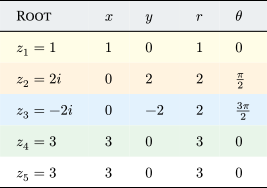
one real root at \(z = (1, 0)\);
one repeated real root at \(z = (3, 0)\); and
one pair of complex conjugate roots at \(z = (0, \pm 2i)\).
Using \(z\) as the variable, our polynomial then becomes: \[(z - 1)(z - 3)(z - 3)(z - 2i)(z +2i) = z^5 - 7z^4 + 19z^3 - 37z^2 + 60z - 36.\qquad{(19)}\]
The Cartesian and polar forms of these five roots are enumerated in Figure 8 below.
To avoid confusion we will define two polynomial functions, one on the real domain and the other on the complex domain. Let the real-valued version be called \(q\) and the complex-valued version be called \(Q\). We then have: \[\begin{aligned} q &: \mathbb{R} \to \mathbb{R}\\ q &: x \mapsto y\\ q(x) &= x^5 - 7x^4 + 19x^3 - 37x^2 + 60x - 36 = y. \end{aligned}\qquad{(20)}\]
Likewise, we define: \[\begin{aligned} Q &: \mathbb{C} \to \mathbb{C}\\ Q &: z \mapsto w\\ Q(z) &= z^5 - 7z^4 + 19z^3 - 37z^2 + 60z - 36 = w. \end{aligned}\qquad{(21)}\]
Plotting the real polynomial \(q(x)\)
We can repeat what we did with the previous example, by plotting the polynomial for the real case, as shown in Figure 9. The single root at \((1, 0)\) intersects the \(x\)-axis at that point, while the repeated root at \((3, 0)\) is tangent to the line \(y = 0\) at that point.
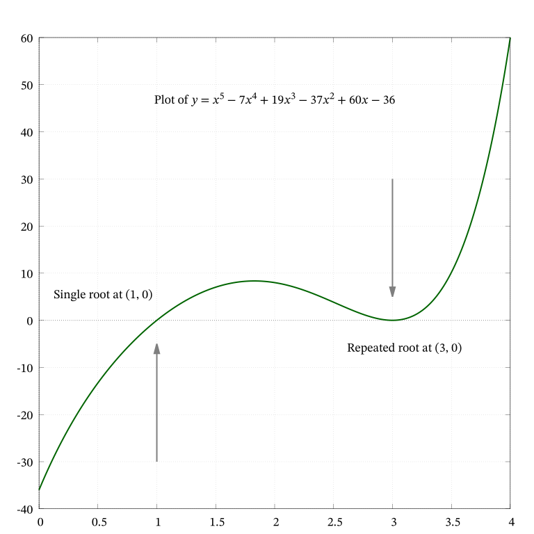
Before considering the complex polynomial \(Q(z)\), I will make a short historical detour to explain how Gauss formulated his first proof of the FTA using the idea of two coupled real polynomials.
Intermezzo: Gauss’s 1799 Proof of the FTA
Gauss used acute observation and crafty manipulation to prove that every complex polynomial \(Q\) of degree \(n > 1\) had at least one complex solution. The arguments of his 1799 (originally disputed) proof—as I have understood them—are sketched out below.
The Paradigm
Finding the roots of any polynomial is the solution of an inverse problem. We know the result, which is zero, and we want to find the cause(s) which is/are the root(s).
So, we start with the zero and backtrack to the roots that gave rise to the zero. For a complex polynomial, there is only one two-dimensional zero point: \((0, 0)\). Because several roots may exist, and since all map to the same zero, the mapping from zero to root is not unique. We are not dealing with an in invertible function.
The Approach
When working with a complex polynomial, \(Q(z)\), Gauss did not mechanically wallow straight into the mire of two complex planes and their four dimensions. Instead he was cautious and circumspect.
He considered the output of the polynomial \(Q\) as a pair: a real polynomial and an imaginary polynomial, coupled by \(i\), but which could be treated as two separate real polynomials, as each behaved independently of the other, but in an orthogonally coupled fashion. This approach enabled profound simplification. Remember that he published his results in 1799. The computing aids we rely on had not been invented then!
A concrete polynomial \(Q(z)\)
Let \(Q(z)\) as defined in Equation 19 be our running example. We will henceforth skilfully weave our way between the complex viewpoint and that of two real polynomials in two variables, while trying to trace the footsteps of Gauss.
Substituting \(z = x + iy\), in Equation 19 we get, after some (careful) computation and rearrangement:22 \[\begin{aligned} Q(z) &= Q(x + iy)\\ &= u(x, y) + iv(x, y) \text{ where}\\ u(x, y) &= x^5 - 7x^4 - 10x^3y^2 + 19x^3 + 42x^2y^2 - 37x^2 + 5xy^4 - 57xy^2 + 60x \\ & - 7y^4 + 37y^2 - 36\\ v(x, y) &= 5x^4y - 28x^3y - 10x^2y^3 + 57x^2y + 28xy^3 - 74xy + y^5 - 19y^3 + 60y \end{aligned}\qquad{(22)}\]
Effectively, we are looking at two real polynomials, \(u\) and \(v\), both of which vary with \(x\) and \(y\) across some input plane which we will call the \(z\)-plane, without the introduction of any third dimension or any mention of a complex plane. As far as this approach is concerned, both \(u\) and \(v\) are polynomials in two real variables.
The Technique
To solve the inverse problem of finding the roots, Gauss needed to prove that these two equations had at least one solution: \[\begin{aligned} u(x, y) &= 0\\ v(x, y) &= 0. \end{aligned}\qquad{(23)}\]
He used a technique that is routinely used to solve a pair of simultaneous equations. Draw the graphs of both curves using the same coordinates and find out whether and where they intersect. All such intersections are roots that evaluate to zero.
Visual depiction
Figure 10 is a graphical depiction of the zero level sets of \(u(x, y)\) and \(v(x, y)\). What does this mean and how does it relate to the roots?
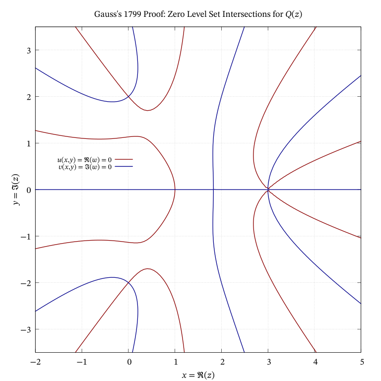
At every point \((x, y)\) on the z-plane, both \(u\) and \(v\) have their own specific values as assigned by \(Q\) as defined in Equation 22. Since we are after the roots, we want those specific points where the two functions are zero as in Equation 23. This act of slicing the output of \(Q\) to give a topographic contour at a particular level is called extracting a level set. In our case, this is a zero level set.
The heavy manual lifting for this is done behind the scenes with little fuss by the Gnuplot plotting program and Figure 10 is the result. It would have would have been seriously burdensome to do it manually.
Gauss was not after the specific roots of any polynomial. Rather, he wanted to prove that every complex polynomial had at least one root. And for this he relied on certain observations. To follow the thread of his logic, we need to cast \(Q(z)\) into its polar form.
Polar parametrization
If you examine Figure 10 closely, you will find the red and blue lines alternating. Is this alternation true for all polynomials? Also, what is its significance? To answer this question, we need to express \(Q(z)\) in polar form, by substituting \(z = re^{i\theta}\) into \(Q(z)\): \[Q(re^{i\theta}) = r^5 e^{5i\theta} - 7r^4 e^{4i\theta} + 19r^3 e^{3i\theta} - 37r^2 e^{2i\theta} + 60re^{i\theta} - 36\qquad{(24)}\]
The profound equation linking the exponential and trigonometric functions and the complex unit \(i\), called Euler’s formula, is: \[e^{i\theta} = \cos\theta + i\sin\theta.\qquad{(25)}\]
A corollary to this formula is that when the LHS is raised to an integer power, \(n\), we have \[e^{i(n\theta)} = \cos(n\theta) + i\sin(n\theta)\qquad{(26)}\] which is called De Moivre’s formula. Note that \(\theta \in \mathbb{R}\) and \(n \in \mathbb{Z}\).
Using Equations 25,26 and separating the real and imaginary parts in Equation 24 we get: \[\begin{aligned} u(r, \theta) &= r^5\cos(5\theta) - 7r^4\cos(4\theta) + 19r^3\cos(3\theta) - 37r^2\cos(2\theta) + 60r\cos(\theta) - 36 \\ v(r, \theta) &= r^5\sin(5\theta) - 7r^4\sin(4\theta) + 19r^3\sin(3\theta) - 37r^2\sin(2\theta) + 60r\sin(\theta) \end{aligned}\qquad{(27)}\]
As before, \(u\) and \(v\) are the polar versions of the real and imaginary polynomials comprising \(Q\).
Behaviour at large \(r\)
What happens to Equation 27 at large values of \(r\)? Imagine a circle of very large radius \(R\) centred on the origin. Recall that rays from the origin of radius \(r\) radiate outward to this circumference, and the angles they make with the positive \(x\)-axis are called \(\theta\) in radians.
Equation 27 tells us that both \(u\) and \(v\) are dominated by the large value of \(R^5\). And because both \(u\) and \(v\) are real polynomials, we have \[\begin{align} u(r, \theta) &= R^5\cos(5\theta) + \text{ terms with smaller powers of $R$}\\ &\approx R^5\cos(5\theta)\\ v(r, \theta) &= R^5\sin(5\theta) + \text{ terms with smaller powers of $R$}\\ &\approx R^5\sin(5\theta)\\ \end{align}\]
There would be one point \(R^5\cos(5\theta)\) on the \(u\)-line. This will be followed by a point \(R^5\sin(5\theta)\) from a \(v\)-line. This means that walking around the periphery of radius \(R^5\), one would encounter a \(u\)-line, followed by a \(v\)-line, followed by another \(u\)-line and another \(v\)-line etc. The spoke-like \(u\) and \(v\) lines would alternate at the periphery as one walked the perimeter.
Why does this happen? Because the \(\cos\) and \(\sin\) functions are in quadrature or \(\frac{\pi}{2}\) radians apart in phase. So, where one is maximum, the other would be zero and vice versa.
This leads to the pattern of alternating red and blue lines that are depicted in Figure 10.
WWWWWWWWWWWWWWWWWWWWWWWWWWWWWWWWWWWWW Because we are trying to prove the FTA—and that too using geometry and topology—the graph of input image circles mapped to output image loops will serve our purpose better than other types of complex function plotting.
WWWWWWWWWWWWWWWWWWWWWWWWWWWWWWWWWWWWWW
From \(z\)-plane to \(w\)-plane using circles
While Gauss got away without considering two planes because of his astute formulation of equations à la Equation ¿eq:poly-two?, the modern technique is to look at complex variables as an orthogonal pair of numbers.
How do we depict the polynomial \(Q(z)\) in Equation ¿eq:poly-two? on the complex plane \(\mathbb{C}\)? We have looked at this issue at some depth with the polynomial \(P(z) = z^2 + 1\) in the previous example. So, I will be brief and to the point here.
This section mirrors what we earlier covered in this blog as Mapping the \(z\) and \(w\)-planes side by side.
This time, because \(Q(z)\) cannot be differentiated everywhere on the \(w\)-plane, we do not have a conformal mapping, but we do have a picture of how input circles on the \(z\)-plane become image loops in the \(w\)-plane. And we would be able to see them all at once, if only we had sufficient resolution.
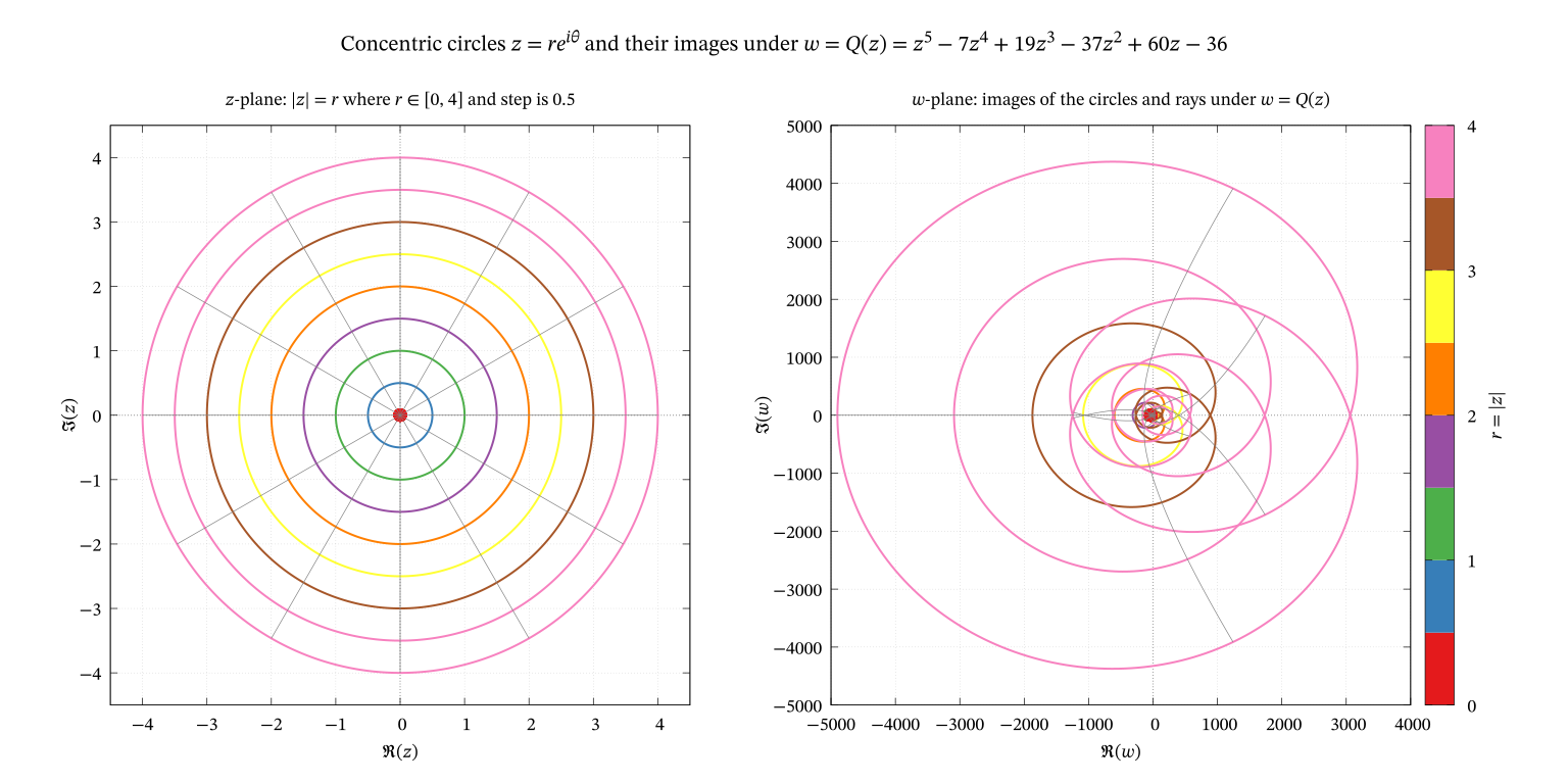
The circular area filled in red in Figure 11 is centred on \((0, 0)\) on the \(z\)-plane and on \((-36, 0)\) on the \(w\)-plane. Note the “circles within circles” or “whorls in a flower” appearance of the image loops on the right panel.
Because the degree of the polynomial is \(5\), the values on the right panel are enormous compared to those on the left for large values of \(r\). One needs to zoom in to see details. The right panel is very cluttered and will be displayed in greater resolution in subsequent sections.
Input circles and output image loops
We now come to our intended depiction of the output \(Q(z) = w\). The polar parametrization allows us freedom to fix one variable and let the other vary. We will keep the value of \(r\) fixed on the \(z\)-plane, and let \(\theta\) vary. The inputs are therefore circles. The output loci are drawn as parametric plots on the \(w\)-plane. We will use the same notation as given in Equation 13.
How does this polynomial behave at very small or very large values of \(r\)? For \(0 < r \ll 1\), the terms involving \(z\) or its higher powers will largely vanish and only the constant, \(-36\) will dominate. For very large values of \(r\), we expect the term involving \(z^5\) to dominate. The order of magnitude will be \(r^5\). Because the polynomial is a continuous function, its image will also be continuous and range over these extremes.
The plot of \(Q(z)\) around the roots, and for very small values, and very large values, are orders of magnitude apart, and difficult to capture on the same plot. So, we have to show them in separate plots for meaningful comparison.
Note that because we constructed \(Q(z)\) to have five roots, it is only for those inputs, shown in Figure 8 that the output will be \(w = (0, 0)\). Only those five, none else. So, the vast majority of output values will be non-zero. Keep Figure 8 in mind as we cycle through the roots hereafter.
The first root at \((1, 0)\)
The plot for small values of \(r\), near the first root, is shown in Figure 12. The output loci for constant input \(r\) are all closed curves as we would expect. These curves may loop but they are guaranteed to close because the trigonometric functions are periodic.
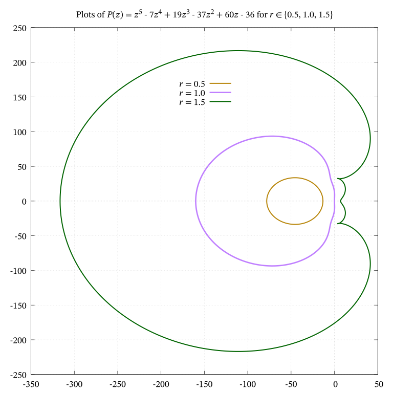
Notice the ripples as well as the loops within loops—almost as if handwritten—as the main curves veer away from the root.
Metaphorically, the root acts as a gravitational source pulling portions of the curve to the origin. Then the curve expands away from the root as \(r\) increases, only to “fall back” into the origin as another root is approached. At all times, though, the outer loop is increasing in size. After the final root has been exited, the curve expands to become very large, and has escaped forever from the “gravity” of the roots.
You might have a nagging doubt about the curves corresponding to \(r\) values like \(1.2\) and \(1.3\) which seem suspiciously close to the origin at \(w = (0, 0)\). Do they too pass through the origin?
To clear those doubts, I have captured a zoomed screenshot of the plots near the origin and shown it as Figure 13 below.
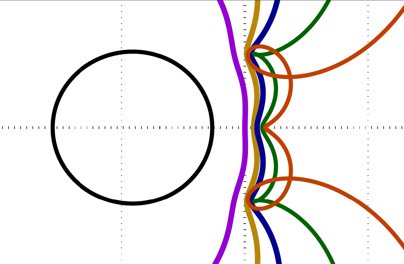
The coefficients of the polynomial and their relative numerical values determine the shape of the curves. The main loop is like a rubber band. The subsidiary loops that cross over the main loop are like parts of a rubber band that double up on the main loop. This happens to “snag” the origin if there is another root. Then the small loops are released. Meanwhile, the main loop keeps on expanding. This behaviour concludes after the last root has been “snagged” and the curve keeps on expanding for increasing \(r\).
The conjugate roots at \((0, \pm 2i)\)
There are four other roots and it is incumbent upon us to examine the output loci carefully for those cases as well.
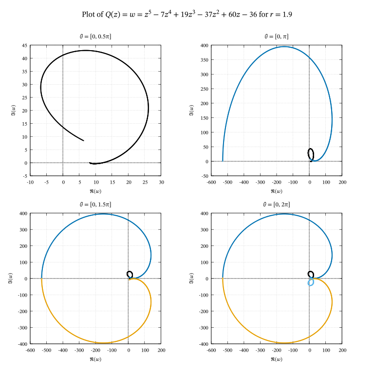
The two conjugate roots at \(z = (0, \pm 2i)\) have \(r = \sqrt{0^2 + 2^2} = 2\). Let us plot the curve for \(r = 1.9\) first. There is a fair bit of “busyness” in the curve around the origin. Does it or does it not pass through the origin? Also, how many times does it cross the real \(u\) axis?
Figure 14 shows the evolution of the curve through four snapshots—for four equally spaced segments of \(\theta\)—each being a quarter of a circle. Moreover, from the four curves corresponding to the four equal intervals of \(\theta\), it is clear that the length of curve associated with an interval of \(\theta\) is not proportional to the interval. Although these curves are closed, they are not simple circles. They may feature cusps, loops, etc.
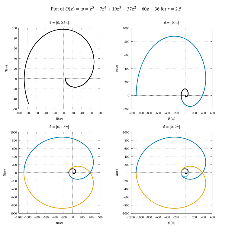
Similar sets of plots are now shown for \(r = 2.0\) and \(r = 2.5\) to highlight the familial evolution of these curves. The curve for \(r = 2.0\) is associated with the two conjugate roots.
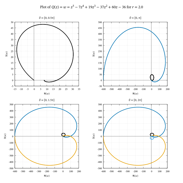
There is no extraordinary change in behaviour between the curves for \(r = 1.9\), \(r = 2.0\), and \(r = 2.5\). In terms of appearance, shapes, etc., it is more of the same. It is only upon close examination that, whether the curve passes through the origin \((0, 0)\) becomes the distinguishing characteristic.
The repeated root at \((3, 0)\)
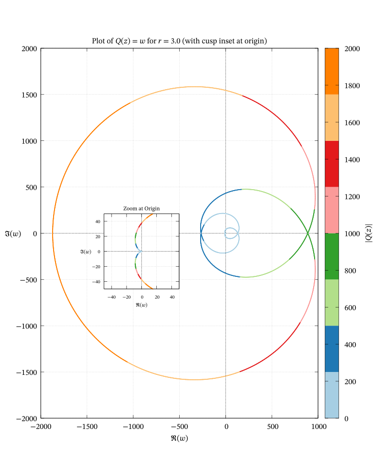
The repeated root at \(z = (3, 0)\) is the last set of roots of \(Q(z)\) that we need to look at. The cusp at \(w = (0, 0)\) is a bridge in the evolution of the curve from \(r = 2.5\) to \(r = 3.0\). Observe how the overall curve keeps expanding while the loops within loops keep pinching to wriggle toward or around the origin before relaxing and moving off to join the main loop. It is a bit like linear ballons being pinched to form animal shapes, except that these shapes are both transient and dynamic with these curves.
Zero crossings again
The trace made by \(Q(z)\) for a given \(r\) on the \(w\)-plane is closed because of the periodicity of the trigonometric functions.
Also, for a polynomial of degree \(n\), this locus winds around \(n\) times for each \(2\pi\) of the input argument because of De Moivre’s formula.
That is why we get the closed curly loops, cusps, limaçons, cardioids, lemniscates, and roses found in polar plots. The interested reader should refer to the OpenStax Precalculus text [7] for more detail on these shapes.
It appears that polynomial roots and zero crossings are an item. Where there is one, the other is bound to be found. But how do we decipher the zero-crossings in complex polynomials, compared to the transparent \(x\)-axis intersections in the real case?
We made a start in Figures 15,16 where the trajectory was coloured according \(\theta\). Even then, the task of tracing the path in a single sweep proved visually difficult and provoked dizziness.
Tracking the zero crossings was, for me, the hardest part of the proof for the FTA. I simply could not be convinced that the zero crossings and winding numbers were what the roots would lead us to expect. Accordingly, I will take up this issue next.
Counting zero crossings
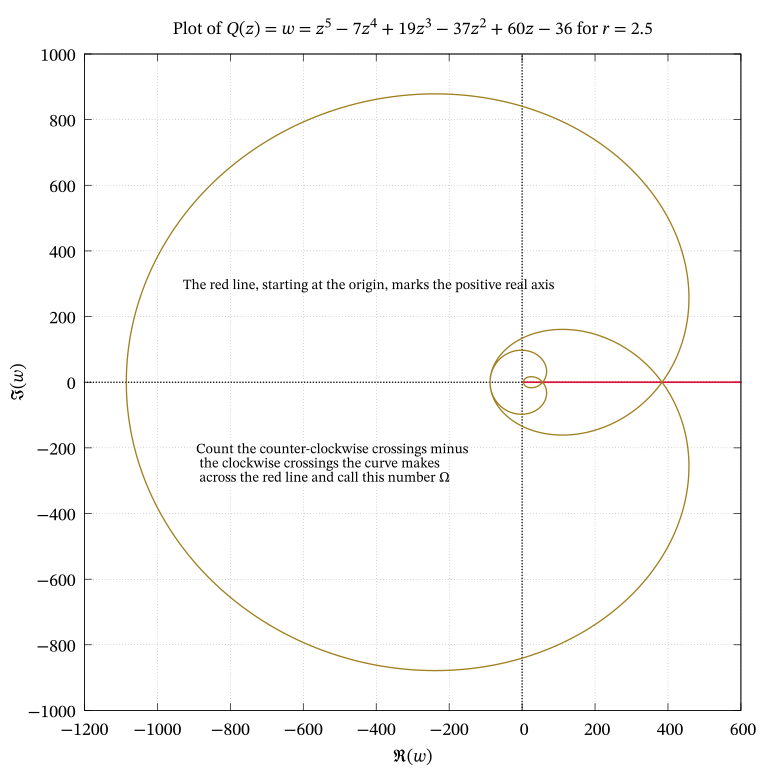
The image loop for \(r = 2.5\) is an image of “whorls within whorls”, not unlike a flower. This makes it taxing visually and mentally to keep track of which whorl we are dealing with or how many times the curve has traversed in which direction.
The vital takeaway is that the completed curve is symmetric about the real axis. If one were to count the number of times the curve goes around the origin counterclockwise minus clockwise, it can make one dizzy. I tried several times before I decided to rely on other means of counting. More on that later.
In the search for roots of polynomial, it seems that we cannot escape certain recurrent themes. I am going to single-step through zero crossings and why they are relevant to our blog on the FTA.
Consider \(r = 2.5\). At this radius, the locus of constant \(r\) is large enough to enclose the root at \((1, 0)\) and the twin conjugate roots at \((0, 2i) and (0, -2i)\)—a total of three roots. How does this pan out on the graph?
Now, if we return to Figure 18, and we start moving right from the origin and count the number of zero crossings the curve makes with the red positive real axis, we can count a total of three. And this number equals the number of roots whose modulus is less than \(r = 2.5\).
If we plot a curve with \(r > 3\), will we encounter a total of five zero crossings? This idea linking the geometry of the complex polynomial curve and its algebraic roots is an intriguing possibility worth exploring.
Colored segments
To assist in this accounting, the image loop in Figure 19has been deliberately colored differently for each quadrant of the input argument \(\theta\) to help track curve evolution.
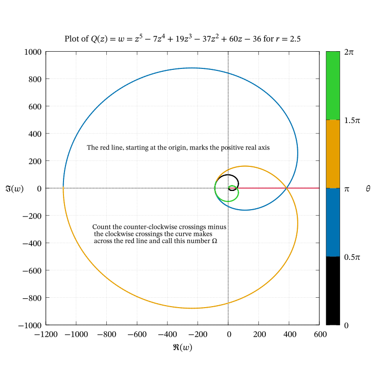
There are certain static features like the symmetry that are immediately apparent, but which can also make counting curve rotations frustratingly difficult. “Return to zero” as in many board games can make this an impossible exercise. It easy to lose track and have to start counting again, close to the finish.
“Vectorizing” the plot
The image loops are symmetrical about the real axis. My mind stubbornly refused to accept that there was some asymmetry that could lead to cancellation of the number of rotations. So, it was decided to attach little vectors, superimposed ion the image loop to help track the direction of the zero crossings.
The next step was to “vectorize” the plot by superimposing small arrows every so often on the curve to unambiguously indicate the direction of the zero crossing. This is shown in Figure 20.
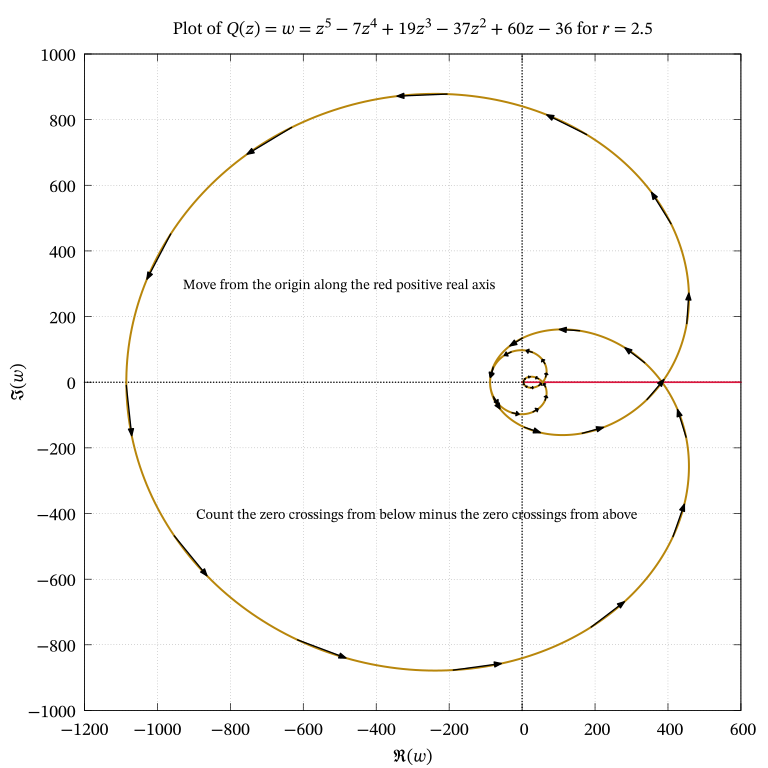
From this plot, it is clear that the loop closest to the origin on the positive crosses the positive real axis from top to bottom. It is the closure enforced by \(\theta = 0\) and \(\theta = 2\pi\).
The total number of zero crossings is, counting from the left on the red line equal to: \(-1 + 1 + 1 + 1 +1 = 3\) and the number of roots “enclosed” by \(r = 2.5\) equals three. We will recall this fact later.
Animation
Rather than view the image loops of \(Q(x)\) in piecemeal fashion, it would help us to visualize the loops as one continuous sequence. And this requires animation.
We have already seen in Figure 7 the output of keeping \(r\) fixed at different values and allowing \(\theta\) to vary over \([0, 2\pi]\). Rather than see such snapshots, I would prefer to show you a movie that ranges over all the values within a fixed interval, say, \(r \in [0, 4]\). This interval was chosen because it includes all five roots, each of which has a modulus less than \(4\).
The excellent Desmos website fortunately allows convenient plotting and animation to help visualize functions geometrically. It also allows animations to be shared via web links. I request you to go there to view some animations I have set up that will hopefully make the curves come alive for you.
Global: closed curve stack
In Animation One we see a sequence of closed curves being shown as \(r\) varies from \(0\) to \(4\). Because the curves are closed, there is no variation with \(\theta\) as the animation cycles through. Whole closed curves are shown for different continuously varying values of \(r\). This is the most complete global view of how the picture of the complex polynomial changes as \(r\) changes.
Be sure to activate the animation and play with the interactive slider of the animation to make it go slow or fast, or freeze it at will. Refer to Figure 8 to remind yourself that all five roots lie within \([0, 4]\), which is the domain of \(r\) specified in the animation.
Watch a few cycles of the curve expanding outwards, being pinched to return to enclose the origin, while still expanding. It is mesmeric dance choreographed by the coefficients of the polynomial in concert with its degree \(n\).
Note that as \(r\) increases, the outer envelope of the image loop also increases. But some portions from within that loop are pinched, rather as in a balloon. It is these internal loops that go toward the origin, touch it, and then go back to the parent loop. All the while, the parent curve is expanding. So, it is not a pulsatile expand-shrink-expand cycle but rather a change in the inner structure of the curve with time.
Obviously, if the upper limit is raised from \(4\) to a larger number, we will see more of the polynomial, but the resolution must become smaller to accommodate the huge values of \(r^5\) that result near the upper limit.
In a sense, this “action movie” of the expanding image loops is the geometric signature of the polynomial. If the continuous evolution of these loops for \(r \in [0, \infty)\) is mapped out, we would have perfectly reconstructed the algebraic equation in visual form.
Of the infinity of points available on the \(w\)-plane, only four unique points give rise to a value of zero.23 Even if an image loop moves suspiciously close to the origin, only these four points give rise to zero output. The roots of a polynomial are extremely rare compared to its input domain.
Local: temporal evolution of a single curve
Let us now look at another animation, this time of a single curve as \(\theta\) changes from \(0\) to \(2\pi\). We fix \(r = 2.5\), and allow \(\theta\) to vary. This is Animation Two. It is the temporal evolution of a single curve. The value of \(r = 2.5\) was chosen as typical of in “between roots” (see Figure 8).
If you concentrate on the origin, you might be suspicious about whether a non-root image loop touches the origin. If in doubt, you may freeze the curve, zoom in, and examine it. From the five roots of Figure 8, we know that only loops with \(r \in \{1, 2, 3\}\) will touch the origin. The mathematics guarantees this.
QUOTE As R grows and passes directly through a root of the polynomial, the entire looping curve transitions—a loop tightly cinches down, crosses through the exact origin (0,0), and opens up on the other side, adding +1 to the overall winding number UNQUOTE
Local: root curves
What about the roots? How do animations of the curves evolve as \(\theta\) changes at the five roots? Refer to Figure 8 to convince yourself that the three values of \(r\) cover all five roots.
Observe the plots at these links, start the animation, and play with the sliders, to see the evolution of the curves as \(\theta\) is varied. If a plot looks minuscule, change the zoom with the mouse wheel to enlarge it.
- Pair of complex conjugate roots at \(r = 2\)
\(z_2 = (x, y) = (0, 2); (r, \theta) = (2, \frac{\pi}{2})\) and
\(z_3 = \overline{z_2} = (x, y) = (0, -2); (r, \theta) = (2, \frac{3\pi}{2})\)
Spatial symmetry and temporal asymmetry
One cognitive-visual trap that I fell into was to confound spatial symmetry with temporal symmetry.
The image loops we have seen are spatially symmetric but temporally asymmetric.
This means when the full curve is frozen in time, it is perfectly symmetric. This is spatial symmetry. Counting turns can get very difficult because the mind militates against any implied asymmetry.
But the curve develops over time asymmetrically. This asymmetry is seen and cannot therefore be denied.
And this makes all the difference in counting the number of counterclockwise turns minus the clockwise turns.
Why all this curve watching?
There is a method behind our madness. This curve watching is directed toward proving the FTA. Gauss carefully observed how these curves wound around the complex origin and struck upon a concept, later known as the winding number, which enabled him to prove the FTA.
So, all this curve watching is for one reason only: to determine the winding number around the origin \((0, 0)\), of the closed curves we have encountered. We define and characterize winding number below.
Winding number
The concept of a winding number straddles the mathematical specialties of topology, geometry, and analysis. It is a powerful unifying idea that simplifies and unites different branches of mathematics. If you wish to pursue this concept in depth, consult the excellent monograph by Roe [8] and the book by Needham [6].
The winding number of a closed curve in the plane—around a given point—is an integer that represents the total number of times the curve travels counterclockwise around that point [9].
Signs
The sign of the winding number indicates the direction of travel:
Positive winding number: The curve winds around the point in a counterclockwise direction.
Negative winding number: The curve winds around the point in a clockwise direction.
Zero: The curve does not wind around the point at all, or the counterclockwise and clockwise turns cancel each other out.
Undefined winding number: The winding number is undefined if the curve passes through the point of interest.
In our case, the constant \(r\)-valued curves from \(Q(z)\) are closed loops on the plane. And the point of interest is the complex origin, \((0, 0)\). Since Gauss used the properties of winding numbers in his proof, it behooves us to look at the winding numbers associated with the image loops of \(Q(z)\), to understand his proof.
The key property of \(Q(z)\) is that, as a polynomial, it is a continuous complex function. And the key topological property of a winding number is this:
The winding number of a continuously varying image loop cannot change unless the loop physically passes through the origin.
Properties
The properties of winding numbers as they apply to the image loops of \(Q(z)\) are summarized below:
The complex origin, \((0, 0)\) is the point around which the windings are counted for the FTA.
The winding number is an integer that is equal to or greater than zero.
The winding number of the curve for any value \(r\) equals the number of roots it encloses.
The winding number is cumulative at any point on the plot, i.e., it does not decrease with increasing \(r\).
For a polynomial of degree \(n\), the winding number stabilizes at \(n\) after all \(n\) roots have been enclosed, and remains so thereafter.
The winding number rings a note of finality to the quest for the roots of a complex polynomial of degree \(n\). After \(n\) roots have been found, no others exist to be found. And this is a vital finding in the quest to tame complex polynomials.
Toplogy and Analysis
The interplay of topology and analysis where winding numbers are concerned is particularly instructive and charming.
Winding numbers are digital or integers because the topology does not admit of a fractional crossing of paths. Paths either cross or do not cross.
Winding numbers are monotonic because polynomials are continuous functions, as guaranteed by analysis.
This means that a plot of winding number against the input radius \(r\) will be like a staircase. Electrical engineers and Physicists deal with such waveforms on a daily basis. At the point of a step—coresponding to a root—the winding number is undefined and corresponds to a singularity, like an impulse function.
A geometric detour
When we plot image loops of \(Q(z)\), we are looking at the geometric definition of the polynomial. To locate roots, we are interested in those values of the input where the output is zero. It is important to note that except for those finite \(n\) input values, the output is non-zero everywhere else.
This sets apart the behaviour at the roots from the behaviour of the polynomial everywhere else. As long as an image loop does not pass through the origin, its value remains defined and one can count the number of times it encircles the origin.
At the origin, this number is undefined and we do not count.
digital monotonicity: digital from topology; monotonicity from algebra
Need to synthesize the whole picture.
Algebraic Closure
Algebraic closure means that the solution to a polynomial lies within the field over which it is defined. The complex field exhibits algebraic closure and this is the kernel of the FTA.
All fields exhibit arithmetic closure, but the complex field also exhibits algebraic closure.
Along the way, the idea of one number being larger or smaller than another was lost.24
Repeated and conjugate roots
When a root \(\rho\) is repeated, the curve for \(r = \rho\) becomes a cusp at the origin.
Moreover, when complex conjugate roots exist, the curve splits into two symmetrical paths that both pass through the origin.
Distinction between arithmetic and algebraic closure
My 4 questions.
Sand and water: real and imaginary
How do we know there are no more roots?
The FTA claims \(n\) roots for a complex polynomial of degree \(n\). But how do we know that the winding number which counts the roots does not increase indefinitely after all \(n\) roots have been found?
This result is guaranteed by two factors:
The dominant terms in \(Q(z)\) for \(0 < \lvert z \rvert < 1\) and for \(\lvert z \rvert\) very large. When \(\lvert z \rvert < 1\), the constant term \(a_0\) dominates the polynomial.25
The “man and dog-on-leash” theorem from Eugène Rouché which uses the triangle inequality to prove a point that is geometrically obvious. If a person were to walk a dog on a leash around and around a tree, such that the distance between the person and the tree is always greater than the length of the leash, then the person and the dog go around the tree the same number of times. And not otherwise.
Rouche’s theorem
Dog on leash? Whose theorem?
Because \(Q(z)\) is a continuous polynomial, it must cross the origin for some \(r\). If small values under-reach it and large values over-reach it, for some value in between the polynomial must evaluate to zero. This capturing the solution on the complex plane is the equivalent of the IVT for the real line.
The technique we have used is the same as what the epsilon-delta definition does to trap a limit within a box,26 or the squeeze theorem in a similar context.
Tie-into Riemann surfaces
This is one solution that works well in certain situations. See the section called logarithms of complex numbers in a previous blog of mine.
“Galois theory is a study of the symmetries both of roots and of their field extensions.” Nathan Carter, Visual Group Theory, Chapter 10.
Scripts for graphical output
The graphs in this blog were generated programmatically. Click on the icon of the graph of interest to you to download the script that generated it.
Acknowledgements
Feedback
Please email me your comments and corrections.
A PDF version of this article is available for download here:
Evolution across the radii https://www.desmos.com/calculator/adqzoihmii
References
Currently, mathematics is morphing into the science of patterns, and who knows what its dominant characteristic will become in the future?↩︎
Only addition and multiplication are defined. See Where have subtraction and division disappeared?.↩︎
I must confess to a certain unease with Dedekind’s logic as, hidden somewhere inside it, is the assumption that the sets of rationals and irrationals are mutually exclusive sets, whose union is the reals. In other words, a dichotomy of the reals was assumed before the proof. Also, it is strange for a proof that claims to untether numbers from geometry to be based on a line of numbers which is “cut”.↩︎
Sometimes also written as \(a + ib\).↩︎
Excluded from this statement are hypercomplex numbers like quaternions, octonions, and sedenions.↩︎
This explains why the roots of polynomials have been so well-studied.↩︎
Or think of it as the intersection of \(y = mx + c\) with \(f(x)\) where both \(m\) and \(c\) are zero.↩︎
Although it takes us to a later part of this blog, note that multiple roots touch—but do not cross—the \(x\)-axis, as shown in Figure 9 for the value \((3, 0)\) on the \(x\)-axis.↩︎
Real variables are traditionally denoted by \(x\) and \(y\) and complex variables by \(z\) and \(w\).↩︎
My only regret is that the 2023 edition did not take advantage of computer graphics to display the diagrams in colour.↩︎
Left Hand Side.↩︎
The symbols \(\Re(z)\) and \(\Im(z)\) are used to denote the real and imaginary parts of the complex number \(z\). The newer practice is to use \(\mathrm{Re}(z)\) and \(\mathrm{Im}(z)\) to denote them respectively. Both forms are in service.↩︎
Zeta, whose lowercase representation is \(\zeta\), is the sixth letter of the Greek alphabet.↩︎
There is yet another method of visualizing complex functions, in which \(P(z)\) is pictured as a vector emanating from \(z\). For more on this profoundly important and practically applicable point-of-view, called a vector field, see Chapters 10 and 11 of Needham [6].↩︎
Note that the modulus of a complex number is sometimes also written as \(\| z\|\).↩︎
Which is a real number.↩︎
If the steps below seem unfamiliar, read my blog A Tetrad of Captivating Problems where the complex exponentials are carefully explained.↩︎
See my blog Gnuplot for the Plotless if you are interested in knowing how this plot was generated.↩︎
See my blog on how monomial power functions behave if you are perplexed by this.↩︎
This covers all the types of roots for polynomials with real coefficients.↩︎
Spare a thought for mathematicians of past centuries who had to do complicated expansions without making an error. In this age of AI, we are spared their travail.↩︎
There are five roots in all, but one is repeated; hence four unique roots.↩︎
The complex field, \(\mathbb{C}\), is not ordered.↩︎
See the section called monomial power functions in my blog The Exponential and Logarithmic Functions if you are unsure why this is so.↩︎
Topological entrapment is the erudite phrase I have heard describing this technique.↩︎