Prelude

This is a sequel to the blog “The Pi of Archimedes”. Here, we look at π as a number—without explicit reference to its geometric tethering—and explore its remarkable ubiquity in mathematics.

As an appetizer, see Figure 1, where the symbol for Pi is surmounted by two very disparate equations defining it. How in all the world could these two different-looking equations be true? But they are indeed!

The Number Menagerie

Numbers may be compared to animals in a zoo. Each is different, and yet they all share some attributes in common. The variety and diversity of zoo animals can be challenging. That is why the big cats are grouped together, the herbivores live in another part of the zoo, etc.

Numbers, like animals, have evolved over many centuries into what I call the number menagerie. A very elementary picture of this zoo is outlined in my blog “The Two Most Important Numbers: Zero and One” in case you need to review some definitions.

To appreciate \(\pi\) as a number, we need to be aware of the taxonomy in the zoo of numbers. It turns out that \(\pi\) is a real number that is transcendental and therefore also irrational. Let us make a short detour to better understand what this means.

Real and Complex Numbers

There are two major sets of numbers: real numbers, denoted by the set \(\mathbb{R}\), and complex numbers, denoted by the set \(\mathbb{C}\). The difference between the two is that while a real number is a single number, a complex number is a pair, composed of two real numbers, conjoined by the imaginary unit \(i\), where \(i^2 = -1\). In set-theoretic notation, we write \[ \mathbb{C} = \{a + bi: a, b \in \mathbb{R}\}. \] Sometimes, the complex number \(a + bi\) is written as the ordered pair \((a, b)\), provided the context is clear.

What then are the reals? The real numbers are the union of the set of rational numbers and the set of irrational numbers. Alternatively, the reals are the union of the algebraic numbers and the transcendental numbers.¹

We will define each of these terms below and how they relate to one another. As always, we start with the known and proceed to the unknown.

The Integers and Friends

The set \(\mathbb{N}\) of natural or counting numbers is defined as \[ \mathbb{N} = \{1, 2, 3, \dots, n, n+1, \dots\}. \] It is a countably infinite set whose members begin with \(1\) and progress by the addition of \(1\) to the predecessor. It is an infinite set, which means it never ends, as denoted by the ellipsis or three dots at the end of the definition.

Zero is not a natural number and is assigned its own, unnamed set, \(\{0\}\).²

The set of integers \(\mathbb{Z}\) includes the negative numbers, zero, and the positive numbers: \[ \mathbb{Z} = \{\ldots -3, -2, -1, 0, 1, 2, 3, \dots\} \] Like \(\mathbb{N}\), \(\mathbb{Z}\) is also a countably infinite set.

A first dichotomy

The real numbers may be partitioned into subsets in different ways: one way is into the rational and irrational numbers.

Every real number is either rational or irrational. If the universe of discourse is the real number set, the rational and irrational numbers are complements of each other. In other words, the union of the set of rational numbers and the set of irrational numbers is the set of real numbers.

Rational Numbers

The rational numbers are denoted by the set \(\mathbb{Q}\) defined to be: \[ \mathbb{Q} = \{\tfrac{a}{b} \mbox{ where } a, b \in \mathbb{Z} \mbox{ and } b \neq 0\}. \] The condition imposed on \(b\) arises from the stricture that division by zero is not permitted among the integers and reals.³

Let us amplify the consequences of these definitions. Is the number \(25\) rational? Yes, indeed. But where is the denominator? It is implicit and equals \(1\). The fact that \[ 25 = \frac{25}{1} \] makes it clear that \(25\) is a rational number. Every integer is a rational number.

And it is obvious from the definition that \(\frac{2}{3}\) is a rational number. But is \(-\frac{11}{16}\) a rational number? Yes, indeed, because the definition depends upon the integer \(a\) and the non-zero integer \(b\), where both integers—being drawn from \(\mathbb{Z}\)—can be signed.

When a rational number is expressed as a decimal, that decimal can either terminate or recur without end.

For example, the fraction \(\frac{1}{3} = 0.\overline{3}\) has a recurring decimal representation as revealed by division. The line on top indicates the portion of the decimal which recurs—in this case, it is the single digit \(3\).

When we look at the fraction \(\frac{1}{2} = 0.5\), we have an example of a terminating decimal. We could, however, pad zeros after the first decimal place, and claim that even a terminating decimal is recurring; witness that \(\frac{1}{2} = 0.5 = 0.5000 \dots = 0.5\overline{0}\). But that is not the whole story.

We can further show that: \[ \frac{1}{2} = 0.5 = 0.5\overline{0} = 0.4\overline{9}. \] It does seem strange to claim that two different decimals can express the same rational number \(\frac{1}{2}\).

To see why, let us rewrite \(0.4\overline{9}\) as \[ \begin{aligned} 0.4\overline{9} = 0.4999\dots &= \frac{4}{10} + \frac{9}{100} + \frac{9}{1000} + \frac{9}{10000}\dots\\ &= \frac{4}{10} + 9\left[ \frac{1}{100} + \frac{1}{1000} + \frac{1}{10000} \dots\right]\\ \end{aligned} \qquad{(1)}\] Consider now the expression in square brackets on the right hand side (RHS) of Equation 1. We can recognize it as a geometric series with first term \(a = \frac{1}{100}\) and common ratio \(r = \frac{1}{10}\). Since \(r < 1\), the series is convergent and its sum to infinity [1] is given by: \[ \begin{aligned} \frac{a}{1 - r} &= \frac{\frac{1}{100}}{[1 - \frac{1}{10}]}\\ &= \frac{\left[\frac{1}{100}\right]}{\left[\frac{9}{10}\right]}\\ &= \left[\tfrac{1}{100}\right] \left[\tfrac{10}{9}\right]\\ & = \tfrac{1}{90}. \end{aligned} \qquad{(2)}\] Substituting for the terms in square brackets in Equation 1, we get \[ 0.4\overline{9} = \frac{4}{10} + 9\left[\frac{1}{90}\right] = \frac{4}{10} + \frac{1}{10} = \frac{5}{10} = \frac{1}{2}. \] Even if it seems counter-intuitive that \(0.4\overline{9} = 0.5 = 0.5\overline{0} = \frac{1}{2}\), it is mathematically consistent and correct. One may therefore hazard a guess, and correctly so, that every rational number may be expressed as a recurring decimal.⁴

Infinite sums have this property of upending our “intuition” about what is correct. So, we have to be extra careful when dealing with the value of a limit as some variable goes to infinity.

Moreover, infinity, represented by \(\infty\), is not a number and cannot be treated as one. It is simply a convenient shorthand symbol. This caveat should be kept in mind when we encounter infinite sums involving \(\pi\), as shown for example, in Figure 1.

Irrational Numbers

Irrational numbers are numbers which are not rational. The discovery that \(\sqrt{2}\)—which is the length of the diagonal of a unit square—was not rational [2–4], caused the first ripples of disquiet in the ancient mathematical world, because it upset the prevailing philosophy that ratios of whole numbers alone ruled the world.

There are many celebrated proofs that \(\sqrt{2}\) is not the ratio of two integers and is therefore irrational [5]. Nevertheless, it took almost two millennia for \(\sqrt{2}\) to be accepted into the fold of properly defined numbers [6].

An irrational number like \(\sqrt{2}\) does not have any recurring sequence of digits when expressed as a decimal. But the absence of recurring sequences in the decimal representation of a number should not solely be used to identify a number as irrational, because some rationals with large denominators can and do have very long recurring sequences, which may be difficult to detect by visual inspection. For example, \(\frac{8119}{5741}\)—which incidentally is a rational approximation to \(\sqrt{2}\)—has a recurring sequence of length \(5740\)!⁵

The irrationals far outnumber the rationals

If you are curious, you might wonder which are the more numerous: the rationals or the irrationals? You might guess that the familiar rationals are more numerous than the obscure irrationals. But you would be mistaken.

In fact, the irrationals far exceed in number the rational numbers [7]. This fact is stated baldly here, because going into the whys and wherefores of this claim will lead us too far astray from our focus on \(\pi\). It is an interesting fact, though, that you should stash away for future investigation.

A second dichotomy

The real numbers may also be split another way into two mutually exclusive sets: the algebraic numbers and the transcendental numbers. Every real number is either an algebraic number or a transcendental number; it cannot be both.

It bears noting though, that both the algebraic and the transcendental numbers may be complex, i.e, have an imaginary part. In this blog, we focus exclusively on real numbers, excluding algebraic and transcendental numbers that involve the imaginary unit.

The Algebraic Numbers

An algebraic number is the root of a non-zero polynomial with integer or rational coefficients. It is the value of the variable when the polynomial equals zero. Things have gotten abstract enough thus far for eyes to be glazed. So, let us invoke some examples to revive attention.

The simplest algebraic number is an integer. Let us take \(5\) as an example. If the polynomial is \(p(x) = x - 5\), its root is the value of \(x\) when \(p(x) = 0\), i.e., when \(x - 5 = 0\), or \(x = 5\). So, \(5\) is algebraic by definition.

Note that we could have used any other polynomial with the same root, such as \(q(x) = 2x - 10\). All we need do is find one polynomial whose root equals the number and we have shown that the number is algebraic.

Likewise, the rational number \(-(\frac{2}{3})\) is the root of the polynomial \(3x + 2\) and is therefore algebraic.

We may assert that every rational number is algebraic and therefore not transcendental.

But what about an irrational number like \(\sqrt{2}\)? Is it algebraic? The polynomial \((x^2 - 2)\) has zeros at \(\pm\sqrt{2}\), thereby demonstrating that both \(\pm\sqrt{2}\) are algebraic.

Can an algebraic number be a complex root of a real polynomial? Let us find the roots for the real polynomial \(x^2 - 10x +34\): \[ \begin{aligned} x^2 - 10x + 34 &= 0\\ (x^2 -10x + 25) + 9 &= 0\\ (x - 5)^2 + 9 &= 0\\ (x - 5)^2 &= -9\\ (x - 5) &= \pm3i\\ x &= 5 \pm 3i\\ \end{aligned} \] We have just shown that an algebraic number can be a complex root of a real polynomial. While we will not consider complex algebraic numbers in this blog, it is useful to know that they do exist.

The Transcendental Numbers

Numbers which are not algebraic are assigned the rather exalted title of transcendental numbers. Numbers like \(\pi\), \(e\), and \(\ln 2\) are transcendental. But proving that a particular number is transcendental is no mean task. We will accept \(\pi\) as transcendental if it has been proved to be so by professional mathematicians [8–10].

All transcendental numbers are perforce irrational.

Transcendental numbers can also be complex, e.g., \(e^{i}\), but we will steer clear of that category here, because we don’t want to get more dizzy (mathematically) than we already are right now! 😉 .

Taxonomy via Tetrachotomy

We have established a tetrachotomy among the real numbers. But the four parts are not mutually exclusive. They overlap. There are two non-overlapping dichotomies: the rationals and irrationals as one pair, and the algebraic and transcendental numbers as the other.

It is noteworthy that irrational numbers like \(\sqrt{2}\) and transcendental numbers like \(\pi\) and \(e\) are denoted, not by values, but by symbols.

This classification of the real numbers seems to be crying out for a Venn diagram to depict it visually. But before we do that, let us marshal the facts we have gathered so far:

1. The real numbers are represented by the standard set \(\mathbb{R}\).

2. The rationals are represented by the standard set \(\mathbb{Q}\).

3. There is no assigned symbol for the set of irrationals. Because it is the set difference between the reals and the rationals, it is often denoted as \(\mathbb{R}\setminus\mathbb{Q}\). But this notation is cumbersome. So, let us define a non-standard set \(\mathbb{I}\) and let it stand for the irrationals: \(\mathbb{I} = \mathbb{R}\setminus\mathbb{Q}\).

4. Let us introduce the non-standard symbol \(\mathbb{A_{\mathbb{R}}}\) for the set of real algebraic numbers.

5. Let us introduce the non-standard symbol \(\mathbb{T_{\mathbb{R}}}\) for the set of real transcendental numbers.

6. The real numbers are the union of the set of rational numbers and the set of irrational numbers: \(\mathbb{R} = \mathbb{Q} \cup \mathbb{I}\).

7. The real numbers are also the union of the algebraic and transcendental numbers that do not embody the imaginary unit \(i\): \(\mathbb{R} = \mathbb{A_{\mathbb{R}}} \cup \mathbb{T_{\mathbb{R}}}\)

8. Algebraic numbers can be either rational or irrational: \(\mathbb{A_{\mathbb{R}}} \subseteq (\mathbb{Q} \cup \mathbb{I})\).

9. All rational numbers are algebraic: \(\mathbb{Q} \subset \mathbb{A_{\mathbb{R}}}\)

10. No rational number is transcendental: \(\mathbb{Q} \cap \mathbb{T_{\mathbb{R}}} = \emptyset\)

11. All real transcendental numbers are irrational: \(\mathbb{T_{\mathbb{R}}} \subset \mathbb{I}\).

12. The irrational numbers contain all transcendental numbers and a subset of the algebraic numbers, again excluding those that embody \(i\): \((\mathbb{T_{\mathbb{R}}} \subset \mathbb{I}) \wedge (\mathbb{A}_{\mathbb{R}} \cap \mathbb{I} \neq \emptyset)\).

That was quite a mouthful even with mathematical symbols. We are now ready to draw the Venn diagram for the tetrachotomy of the real numbers.

And surprise! surprise! There are only three regions in the Venn diagram that are populated. So, taking mathematical liberties, we may say that our tetrachotomy was not “linearly independent”.

Enter π

Pi is not only important, it is also tantalizing. It is like a beautiful butterfly that cannot be caught in the net of finitude. It is like a rainbow that is beautiful to behold from afar, but can never be touched.

It is not a rational number, which means that it cannot be expressed as the ratio of two whole numbers, the denominator being non-zero. Its decimal representation is neither finite nor does it contain a recurring segment. It is also not the root to any polynomial equation whose coefficients are integers or rational numbers. Pi thus qualifies as a transcendental, irrational number.

We have gone through all this huffing and puffing to place \(\pi\) contextually among the real numbers. Let us list its characteristics:

1. It is not a rational number, which means that it cannot be expressed as the ratio of two whole numbers, the denominator being non-zero.

2. Its decimal representation is neither finite nor does it contain a recurring segment, regardless of how long the decimal is.

3. It is also not the root to any non-zero polynomial equation whose coefficients are integers or rational numbers.

4. When Pi is used in equations, the placeholder symbol \(\pi\) is used.

One could claim that \(\pi\) is not numerically friendly. And you would not be too wrong. Rational approximations for \(\pi\), like \(\frac{22}{7}\), are used in practice. And the matter would have rested there were it not for the human quest for accuracy and beauty.

The unpredictability of successive decimal places of \(\pi\) has enchanted mathematicians and still continues to engross them. Pi has been calculated to an unprecedented number of decimal places, and such a quest is certainly driven, not by practical necessity, but possibly by the need for aesthetic fulfilment.

There is also a tacit belief among some that the digits of \(\pi\) might conceal within themselves the secret of what it truly means to be random.

The search for increasingly more accurate values for \(\pi\) has resulted in many approaches to solve the problem. Geometric⁶ and analytical approaches to estimate \(\pi\) have both borne fruit. Interestingly, \(\pi\) may also be estimated by repeatedly performing a random—or probabilistic—experiment, whose precise outcome cannot be predicted, but whose average behaviour may be estimated. Such an experiment is called a Monte Carlo simulation. Thus the quest for \(\pi\) brings together the mathematical sub-fields of geometry, analysis, and probabilistic simulation.

This quest for the unattainable—but supremely beautiful—has engaged human minds to seek \(\pi\) in countless infinite sums, such are shown in Figure 1. These equations are sometimes starkly simple and at other times thoroughly mystifying. They embody the paradox that is \(\pi\) more succinctly than all the words and numbers in the world.

Ludolph van Ceulen and François Viète

Before we set sail to explore \(\pi\) further, let us indulge in one last glance at The Pi of Archimedes and how the work of two mathematicians—who lived in the latter half of the 1500s—formed a bridge from the polygon method of Archimedes to newer infinite series methods for estimating this transcendental number.

Ludolph van Ceulen [11] is one of the unsung heroes in the perennial quest to calculate ever more digits of \(\pi\). He faithfully and heroically followed in the footsteps of Archimedes and spent almost twenty-five years of his life to evaluate \(\pi\) to 35 decimal places⁷ [11,12]. It is fitting that his restored tombstone in Leiden is inscribed with the upper and lower bounds of \(\pi\) [13] that he so painstakingly computed:

π > 3.14159265358979323846264338327950288
π < 3.14159265358979323846264338327950289

François Viète not only emulated the polygonal approach of Archimedes to estimate \(\pi\), but also introduced algebraic notation [14,15] to allow for greater abstraction. Even more significantly, he introduced—for the first time—an explicit, infinite product formula for the exact value of \(\pi\), now known as Viète’s formula [15,16], consisting of a product of nested radicals: \[ \begin{aligned} \frac2\pi &= \frac{\sqrt 2}2 \cdot \frac{\sqrt{2+\sqrt 2}}2 \cdot \frac{\sqrt{2+\sqrt{2+\sqrt 2}}}2 \cdots\\ \frac2\pi &= \prod_{n=1}^{\infty} \cos \frac{\pi}{2^{n+1}}. \end{aligned} \qquad{(3)}\] Eli Maor has observed that:

“Viète’s formula marks a milestone in the history of mathematics: it was the first time an infinite process was explicitly written as a succession of algebraic operations. … By adding the three dots at the end of his product, Viète, in one bold stroke, declared the infinite a bona fide part of mathematics. This marked the beginning of mathematical analysis in the modern sense of the word.” [15].

While van Cuelen’s work displayed superhuman effort and dedication, it also demonstrated that the method of Archimedes did not converge rapidly to \(\pi\). Viète’s formula bridges the divide between the ancient and the modern by embodying \(\pi\) and infinity for the first time in an explicit and exact equation, allowing more and more efficient estimates of \(\pi\) to be uncovered in due course.

The Madhava-Gregory-Leibniz series

It must be obvious by now that trigonometry, circles, and the number \(\pi\) are inextricably entwined.⁸ The quest for more accurate values of \(\pi\) continued to fascinate mathematicians in the centuries after Archimedes. This time though, rather than geometric iteration, sums of successive terms were used to approximate \(\pi\).

For our purposes, a sequence is an ordered procession of numbers, and a series is a sum of successive terms that obey some specific rule. If the summation stops at some particular term, we have a partial sum; if the summation goes on indefinitely, we have an infinite series. If this infinite sum approaches ever closer to a finite value, the series is said to converge. To see what all this means in practice, let us look at the Madhava-Gregory-Leibniz series.

Why a triple-barrelled name?

The series we are about to look at was originally called the Gregory series. Leibniz evaluated the Gregory series for a specific value and came up with a formula for \(\pi\), and that series was called the Leibniz series.

The accomplishments of medieval Indian mathematicians—whose discoveries antedated those of Gregory and Leibniz—remained unknown to the larger world. But recent scholarship has accorded priority to the leading Indian mathematician-astronomer of that period, Madhava, who anticipated both the Gregory series and the Leibniz series by more than 250 years [17–21]. This explains the triple-barrelled name for the series. Thumbnail sketches are given in the links below for all three mathematicians.

James Gregory was the first Professor of Mathematics at the University of Edinburgh and in 1671, he published the series that was called the arctangent series,⁹ or the Gregory series.

Gottfried Wilhelm Leibniz evaluated the arctangent series at \(\frac{\pi}{4}\) to get an estimate of \(\frac{\pi}{4}\); the result was known as the Gregory-Leibniz series or the Leibniz Formula.

Madhava of Sangamagrama was a mathematician-astronomer who pursued research in trigonometric power series. In this, he showed remarkable prescience in defining angular measure as the ratio of arc length \(s\) to radius, \(r\), thus establishing the naturalness of radian measure for serious work in trigonometry.¹⁰

Derivation

Rather than draw the Madhava-Gregory-Leibniz (here abbreviated as the MGL) series out of a hat, we will sketch its derivation, according to Gregory, and show its origins in integral calculus.

We assert that \[ \int_{0}^{x}\frac{1}{1+ t^2}{\mathrm{d}} t = \arctan{x} \qquad{(4)}\]

This integral should be familiar to most high school students. If it is not, try substituting \(t = \tan \theta\): \[ \begin{array}{rcl} t & = & \tan \theta \quad \mbox{ which gives} \\ \displaystyle \frac{\mathrm{d}t}{\mathrm{d}\theta} & = & \displaystyle \frac{\mathrm{d}}{\mathrm{d}\theta}\left[ \tan \theta \right] \\ & = & \sec^2 \theta \\ & = & 1 + \tan^2 \theta \\ & = & 1 + t^2\\ \mbox{Therefore}\quad\frac{1}{1 + t^2}\mathrm{d} t & = & \mathrm{d}\theta\\ \end{array} \]

The integral of Equation 4 now becomes \[ \begin{array}{rcl} \displaystyle \int_{0}^{x}\frac{1}{1+ t^2}\mathrm{d}t % & = & \displaystyle \int_{\arctan0}^{\arctan x} \mathrm{d}\theta\\[1em] & = & \big[ \theta\big]^{\arctan x}_{\arctan0} \\[1em] & = & \arctan x \end{array} \qquad{(5)}\]

This takes care of the right hand side of Equation 4. If we performed long division on the left hand side of the same equation, we get: \[ \begin{array}{rcl} \displaystyle \int_{0}^{x}\frac{1}{1+ t^2}\mathrm{d}t % & = & \displaystyle \int_{0}^{x}% \left[ 1 - t^2 + t^4 - t^6 +\dots \right] \mathrm{d}t \\[1em] & = & \displaystyle \left[ t - \frac{t^3}{3} + \frac{t^5}{5} - \frac{t^7}{7}+ \dots \right]_{0}^{x}\\[1em] & = & \displaystyle x - \frac{x^3}{3} + \frac{x^5}{5} - \frac{x^7}{7}+ \dots \end{array} \qquad{(6)}\]

Using Equations 5, 6, we get the Madhava-Gregory series \[ \arctan x = x - \frac{x^3}{3} + \frac{x^5}{5} - \frac{x^7}{7} + \dots \qquad{(7)}\] Notice that it is only a small step from here to substitute \(x = 1\)—because \(\tan\frac{\pi}{4} = 1\)—to get the equation \[ \begin{array}{ccccc} \arctan 1 & = & \frac{\pi}{4} & = & 1 - \frac{1}{3} + \frac{1}{5} - \frac{1}{7} + \dots \\[0.5em] & & \pi & = & 4(1 - \frac{1}{3} + \frac{1}{5} - \frac{1}{7} + \dots) \end{array} \qquad{(8)}\] which is the MGL series, that is also shown at the top of Figure 1. Strangely, Gregory did not publish the special case of Equation 8, and it was Leibniz who discovered both Equations 7, 8 in 1674, and published them in 1682. For details of Madhava’s terminology and approach, do consult the literature [17–20]. It is noteworthy that Equation 8 was the first infinite series ever found for \(\pi\). However, it converges very slowly. “Calculating π to 10 correct decimal places using direct summation of the series requires precisely five billion terms…” [22].

The Quest for faster convergence

Over the last 370 years, by far the most effort has been expended in discovering series that converge rapidly to \(\pi\), so that even a partial sum of only a few terms will provide an accurate estimate of \(\pi\). We now consider a selection of famous formulae from mathematicians who have bequeathed series for calculating \(\pi\) efficiently.

Machin’s Formula

John Machin followed in the footsteps of the Madhava-Gregory-Leibniz series, but he used the sum or difference of the arctangents of two values to arrive at a more rapidly convergent series for \(\pi\). To better understand his method, let us recall that if \(\tan A = \frac{a_1}{b_1}\) and \(\tan B = \frac{a_2}{b_2}\), then [23]: \[ \begin{aligned} \tan(A + B) &= \frac{\tan A + \tan B}{1 - \tan A\tan B}\\ &= \frac{\frac{a_{1}}{b_{1}} + \frac{a_{2}}{b_{2}}}{1 - \frac{a_{1}a_{2}}{b_{1}b_{2}}}\\ &= \frac{a_{1}b_{2} + a_{2}b_{1}}{b_{1}b_{2} - a_{1}a_{2}}\\ \end{aligned} \] Notice that \[ \begin{aligned} \arctan\tan(A+B) &= (A + B) \mbox { which implies}\\ \arctan\frac{a_1}{b_1} + \arctan\frac{a_2}{b_2} &= \arctan\left[\frac{a_{1}b_{2} + a_{2}b_{1}}{b_{1}b_{2} - a_{1}a_{2}}\right]\\ \end{aligned} \qquad{(9)}\]

Suppose we set \(a_{1} = a_{2} = 1\), then, Equation 9 we get these sum and difference formulae: \[ \begin{aligned} \arctan\frac{1}{b_1} + \arctan\frac{1}{b_2} &= \arctan\left[\frac{b_{1} + b_{2}} {b_{1}b_{2} - 1}\right]\\ \arctan\frac{1}{b_1} - \arctan\frac{1}{b_2} &= \arctan\left[\frac{b_{1} - b_{2}} {b_{1}b_{2} + 1}\right] \end{aligned} \qquad{(10)}\]

Machin knew all four \(\arctan\) formulae shown below: \[ \begin{aligned} \frac{\pi}{4} &= \arctan\frac{1}{2} + \arctan\frac{1}{3}\\ \frac{\pi}{4} &= 2\arctan\frac{1}{2} - \arctan\frac{1}{7}\\ \frac{\pi}{4} &= 2\arctan\frac{1}{2} - \arctan\frac{1}{7}\\ \frac{\pi}{4} &= 4\arctan\frac{1}{5} - \arctan\frac {1}{239} \end{aligned} \qquad{(11)}\] Note that the rational arguments of the \(\arctan\) functions on the RHS of these equations all have a numerator of one. Henceforth, whenever we talk of the two-term Machin-like formulae we implictly mean these rational fractions with a numerator of one.

Specifically, Equation 12 is referred to as the Machin-formula: \[ \frac{\pi}{4} = 4\arctan\frac{1}{5} - \arctan\frac {1}{239} \qquad{(12)}\] Because \(\frac{1}{5} = \frac{2}{10}\), the first term on the RHS, and its powers, are well suited for decimal calculation by hand. And because \(\frac {1}{239}\) has a large denominator, it converges rapidly. Accordingly, Machin was able to compute \(\pi\) to one hundred decimal places [24] using the first 21 terms.

My questions

But what made Machin choose these particular numbers in Equation 12? I have sought the answer(s) to this vital question from many quarters [25] without much success.

Was the historical process of discovery serendipitous, or was it directed by knowledge that led straight to it? Even if historically serendipitous, is there a systematic and simple route that can today deliver the four two-term Machin-like formulae, much like a can of Coke is delivered from a vending machine when the requisite coins are inserted?

How many ways are there of looking at this one problem? Pythagorean Triples? Gaussian Integers? Nested Square Roots? Trial and Error in a restricted domain?

What was the unifying thread that enabled Størmer to claim in his 1899 paper [26] that there were four and only four Machin-like formulae with two terms?

If and when I find satisfying answers to my questions, I will write about them in a separate, dedicated blog. Meanwhile, if any reader of this blog can throw light on the answers to my questions, I kindly request him or her to email me.

Different routes to π

We now look at how Newton, Euler, Gauss, and Ramanujan each approached the problem of estimating \(\pi\). Like all self-driven geniuses, each of them hewed his own independent path, and the fact that the same destination was reached each time is testimony to the unimaginable mathematical riches that lie buried, waiting to be explored by prepared minds in the future.

Newton, π, and the Binomial Theorem

We know that the area of a unit circle is \(\pi\) square units. If we could use calculus to compute the area of a unit circle, we would have a very handy way to compute \(\pi\). Take a look at Figure 4 and Equation 13, both of which suggest how this could be done:

\[ \frac{\pi}{4} = \displaystyle\int_0^1\sqrt{1-x^2}\;\mathrm{d}x \qquad{(13)}\]

So near and yet so far

But how do we integrate \(\sqrt{1-x^2}\)? If we went the trigonometric substitution route, we would end up literally going in circles, rather than computing a numerical value of \(\pi\). Is there any way we may expand the expression under the square root?

The term \({(1 - x^2)}\) is binomial. Isaac Newton is credited with discovering the binomial theorem in Europe,¹¹ but that theorem was originally shown to be valid only for expressions where the binomial is raised to a positive integer power, e.g., \[ (1 + x^2)^3 = x^6 + 3x^4 + 3x^4 +1. \] Note that we have a polynomial with a finite number of terms on the RHS. This application of the binomial theorem falls squarely in the domain of algebra. The coefficients of the expansion are also known easily and beforehand as entries in Pascal’s triangle.

But \(\sqrt{1 - x^2} = (1 - x^2)^{\frac{1}{2}}\), while also being a binomial expression, is raised to a fractional rather than integral power. Does its expansion have a finite number of terms? And how do we know what the coefficients of the various terms are?

Extending the binomial theorem

The mathematician Steven Strogatz has written a charming essay on this subject in Quanta Magazine [27]. It recounts how a young Newton made an inspired and imaginative leap of faith, and gingerly attempted to extend his own pathbreaking binomial theorem to non-integral powers, to derive the binomial series. After first attempting to estimate the area under the curve, he went on to define the curve itself using his newly devised binomial series. In the process, he had moved from algebra (finite polynomials) to analysis (infinite series). When the results justified his extrapolation, he could estimate \(\pi\) using the newfound relationships.

Once again, this episode exemplifies how mathematics is, at heart, an exploratory science, that does admit of experimentation, and in which logical correctness grants the ultimate seal of approval and acceptance. Mathematics is constantly revised and enlarged through this process of constant re-greening.

Using the binomial series

The binomial series for \((1 - x^2)^{\frac{1}{2}}\) is: \[ \begin{aligned} (1 - x^2)^{\frac{1}{2}} &= \sum^{\infty}_{n=0}\binom{\frac{1}{2}}{n}\;(-x^2)^n\\ &= 1 - \frac{1}{2}x^2 - \frac{1}{8}x^4 - \frac{1}{16}x^6 - \frac{5}{128}x^8 - \frac{7}{256}x^{10} - \cdots \end{aligned} \qquad{(14)}\] The series is supposed to converge for \(\lvert{x}\rvert < 1\). It is therefore sensible to integrate to an upper limit less than \(1\), as indicated in Figure 5.

Using the equations shown in Figure 5, and plugging in the values from Equation 14, we get: \[ \begin{aligned} \pi &= 12\left(\int_{0}^{0.5}\sqrt{1 - x^2}\; \mathrm{d}x - \frac{\sqrt{3}}{8} \right)\\ &\approx 12 \left(\left[x - \frac{1}{6}x^3 - \frac{1}{40}x^5 - \frac{1}{112}x^7 - \frac{5}{1152}x^9 - \frac{7}{2816}x^{11} \right]_{0}^{0.5} - \frac{\sqrt{3}}{8}\right)\\ &\approx 3.1415954446070984 \text{ which is correct to 5 decimal places of }\pi\\ \end{aligned} \]

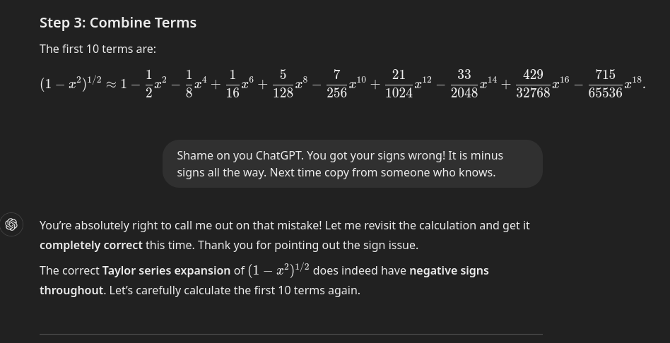
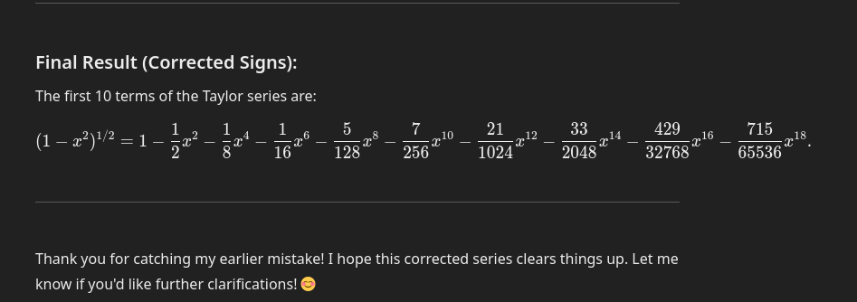
An amusing aside with ChatGPT

I wanted an independent machine check of my binomial series expansion of \((1 -x^2)^{\frac{1}{2}}\) and decided to try out ChatGPT. When I asked it to evaluate the first ten terms of the binomial series of \((1-x^2)^{\frac{1}{2}}\), it gave me a result, all of whose terms did not have the same sign.

After re-checking my computation, I sent it a sardonic message saying that it had erred. Imagine my amazement, when—most human-like—it apologized for its error, and gave me the correct result. The screenshots below show this rather hilarious exchange and underscore the fact that AI is almost human in its responses but its computational side could be beefed up a bit. It also raises the loaded question of whether the ChatGPT error the first time round was deliberate.

Euler’s solution to the Basel Problem

Leonhard Euler is an illustrious polymath among mathematician-polymaths [28]. One of his less celebrated contributions is his solution to the Basel Problem [29] in 1734—eighty-four years after it was posed—when Euler was a mere twenty-eight years old.

The Basel Problem asked for the exact sum of the infinite series of the squares of the reciprocals of the natural numbers. It is perhaps much better expressed and understood in mathematical notation. What is the value of the sum: \[ \sum_{n=1}^\infty \frac{1}{n^2} = \frac{1}{1^2} + \frac{1}{2^2} + \frac{1}{3^2} + \cdots = \mbox{ ?} \]

Euler’s answer was: \[ \sum_{n=1}^\infty \frac{1}{n^2} = \frac{1}{1^2} + \frac{1}{2^2} + \frac{1}{3^2} + \cdots = \frac{\pi^2}{6}. \qquad{(15)}\] His proof was challenged when first presented, but accepted later, in 1741.

What I find fascinating about Equation 15 is that the left-hand side (LHS) is entirely the sum of rational numbers while the sum on the right-hand side (RHS) is irrational. And yet we have exact equality of both sides, not to mention the unexpected closed form of the sum being \(\tfrac{\pi^2}{6}\). How come?

This is the mind-twisting paradox of infinity. I like to think that infinity is where the rationals meet the irrationals. And this equation is not unique in displaying this characteristic. Countless other identities exhibit this same paradoxical property of an infinite sum of rationals exactly equalling an irrational number.

Thus Euler not only gave us another way of computing \(\pi\), but he also showed how elegantly the rationals could dovetail into the irrationals in entirely surprising ways, whenever infinity is involved.

Gauss, the AGM, and π

Carl Friedrich Gauss [30] was a precocious mathematician [31] who published his groundbreaking work only when it met his high standards for terse beauty. Accordingly, many of his contributions became public only many decades after his demise. The material in this section belongs to that category.

I was not aware what the Arithmetic-Geometric Mean (AGM) was until I stumbled upon how Gauss related it to \(\pi\). And he found the connection when he was only 22 years old. So, we are looking at the work of a mathematical prodigy, portions of which are seriously non-trivial.¹²

Accordingly, there will be a lot of hand-waving in what follows, as we attempt a thumbnail outline of Gauss’s method. There are three basic ideas:

1. Lemniscate of Bernoulli;

2. Elliptic integrals; and

3. Arithmetic-Geometric mean (AGM) of two positive real numbers.

By tying together these three ideas, Gauss was not only able to arrive at a potent method of rapidly computing \(\pi\) to high accuracy, but he also opened up new vistas for further mathematical investigation. Our treatment here is sketchy by design and the interested reader is referred to source material for a more complete exposition [32–34].

The Lemniscate of Bernoulli

The Lemniscate of Bernoulli looks like a ribbon tied into a bow, or like the mathematical symbol for infinity. It is a polar curve defined as the locus of points such that the product of distances from two fixed points \((-a, 0)\) and \((a, 0)\) is constant and equals \(a^2\) [35]. Its equation is: \[ \begin{aligned} (x^2 + y^2)^2 &= 2a^2(x^2 - y^2)\; \text{or in polar form}\\ r &= a\sqrt{\cos2\theta} \; \text{where}\; \textstyle{-\frac{\pi}{4} < \theta < \frac{\pi}{4}\; \text{and}\; \frac{3\pi}{4} < \theta < \frac{5\pi}{4}}. \end{aligned} \]

The perimeter is an elliptic integral

It is known that \[ \frac{\mathrm{d}}{\mathrm{d}x} \mathrm{​arcsin}(x) = \frac{1}{\sqrt{1 - x^2}} \] Thus, the integral is \[ \begin{aligned} \int_0^1 \frac{1}{\sqrt{1 - x^2}}\;\mathrm{d}x &= \bigl[\mathrm{arcsin}(x)\bigr]_0^1\\ &= \mathrm{arcsin}(1) - \mathrm{arcsin}(0)\\ &= \frac{\pi}{2}. \end{aligned} \] This implies that: \[ \begin{aligned} \pi &= 2\int_0^1 \frac{1}{\sqrt{1 - x^2}}\;\mathrm{d}x \approx 3.141592653589793. \end{aligned} \qquad{(16)}\] The RHS of equation Equation 16 can be interpreted as the ratio of the perimeter of a unit circle to its diameter.

For the Lemniscate of Bernoulli, the ratio of the perimeter to the diameter (akin to \(\pi\) for a circle) is: \[ \begin{aligned} \varpi = 2\int_0^1 \frac{1}{\sqrt{1 - x^4}}\;\mathrm{d}x \approx 2.622057554292119. \end{aligned} \qquad{(17)}\] The symbol \(\varpi\) is the lemniscate constant \(\varpi\) and is really a variant of the lowercase Greek \(\pi\).

Note that the integral on the RHS of Equation 17 is called an elliptic integral of the first kind.

The family resemblance in these two equations—Equation 16 and Equation 17—is striking, and Gauss looked at their ratio: \[ \displaystyle\frac{\pi}{\varpi} = \frac{2\displaystyle\int_0^1 \frac{1}{\sqrt{1 - x^2}}\;\mathrm{d}x}{2\displaystyle\int_0^1 \frac{1}{\sqrt{1 - x^4}}\;\mathrm{d}x}. \]

The value of the RHS could be computed from first principles, and thus the ratio was known numerically. It is: \[ \frac{\pi}{\varpi} \approx \frac{3.141592653589793}{2.622057554292119} \approx 1.198140234735592. \qquad{(18)}\]

We will now take a look at the third piece of the puzzle, the AGM, before resuming our mathematical tale.

The Arithmetic-Geometric Mean

The arithmetic mean of two numbers \(a_0\) and \(g_0\) is half their sum, \(\frac{a_0 + g_0}{2}\), while the geometric mean of these same numbers is the square root of their product, \((a_0g_0)^{\frac{1}{2}} = \sqrt{a_0 g_0}\). The arithmetic-geometric mean (AGM) of a pair of numbers is a pas de deux of the two numbers obeying the recurrence relation: \[ a_{n+1} = \frac{a_n + g_n}{2}\\ g_{n+1} = \sqrt{a_n g_n} \] As \(n\) increases, the values \(a_n\) and \(g_n\) converge to a common value within a few iterations. This common value is the arithmetic-geometric mean, denoted as \(M(a_0, g_0)\). It has been proved that both \(a_n\) and \(g_n\) converge to the same value denoted by \(M(a_0, g_0)\). [33,36]

For reasons best known to him, Gauss chose to compute the AGM of the numbers, \(a_0 = \sqrt{2}\) and \(g_0 = 1\). Let us follow in his footsteps: \[ \begin{aligned} a_1 = \frac{a_0 + g_0}{2} = \frac{\sqrt{2} + 1}{2} = 1.207106\\ g_1 = \sqrt{\sqrt{2} \times 1} = 1.189207 \end{aligned} \]

A simple script in Julia is available here and may be used to compute the AGM of any pair of positive real numbers. The AGM for \(a_0 = \sqrt{2}\) and \(g_0 = 1\) converges rapidly as shown below.

n a_n                         g_n
0 1.4142135623730951454746219 1.0000000000000000000000000
1 1.2071067811865474617150085 1.1892071150027210268973477
2 1.1981569480946343553284805 1.1981235214931200694365998
3 1.1981402347938772123825402 1.1981402346773073475105775
4 1.1981402347355922799465588 1.1981402347355922799465588

When the above values are compared with those tabulated in Example 2 of the paper by Cox [33], there are discrepancies after 16 decimal places. To check whether better agreement could be achieved by using greater numerical precision in the computation, a second script, agm-big-float.jl was also executed. These results now agree to 19 decimal places with those in the paper.¹³

n a_n                         g_n
0 1.4142135623730950488016887 1.0000000000000000000000000
1 1.2071067811865475244008444 1.1892071150027210667175000
2 1.1981569480946342955591722 1.1981235214931201226065856
3 1.1981402347938772090828789 1.1981402346773072057983838
4 1.1981402347355922074406313 1.1981402347355922074392137
5 1.1981402347355922074399225 1.1981402347355922074399225

So, we may assert: \[ M(\sqrt{2}, 1) = 1.1981402347355922074399225. \qquad{(19)}\]

Comparing Equation 18 and Equation 19 it is clear that their numerical results agree up to the sixteenth decimal place. The fact that two computations from two very different directions—mathematically speaking—have led to the same result, is unexpected to say the least. Gauss was astounded. But unlike most people, he went on to prove that the two expressions on the left hand side of these equations are indeed equal, not just numerically, but mathematically too: \[ \frac{\pi}{\varpi} = M(\sqrt{2}, 1) \qquad{(20)}\] The astute reader would have noticed that the AGM converges rapidly [36]. It is therefore a valuable tool for estimating mathematical constants to high accuracy in a few steps, if such relationships do exist and can be proved. And this was the great insight that resulted from Gauss’s investigation [36].

Gauss wrote in his diary in 1799, after he verified Equation 20, this entry (translated from the Latin into English):

We have established that the arithmetic-geometric mean between \(1\) and \(\sqrt{2}\) is \(\frac{\pi}{\varpi}\) to the eleventh decimal place; the demonstration of this fact will surely open an entirely new field of analysis. [33]

Simply discovering an uncanny agreement between two ways of stating the same thing does not necessarily make for good mathematics. But Gauss went on to prove that an AGM and an elliptic integral were indeed related and equal [37]. That proof is what makes him a great mathematician, and his discovery, great mathematics. And in the process, he enriched mathematics itself.

Why but O! why?

One wonders why Gauss chose \(\sqrt{2}\) and \(1\) as his arguments for the AGM. It was that choice that led to the serendipitous equality to the ratio \(\frac{\pi}{\varpi}\). Does chance only favour the prepared mind [38], and guide it to choose randomly, but with uncanny prescience, something that heralds a discovery? Like Alexander Fleming and penicillin [39]?

Unexpected links between different mathematical sub-fields are discovered by mathematicians who experiment and keenly observe their results. One is reminded here also of James Clerk Maxwell boldly asserting that he could “scarcely avoid the inference that light consists in the transverse undulations of the same medium which is the cause of electric and magnetic phenomena,” [40] upon realizing that the speed of electromagnetic waves and those of light were close. Such leaps of the imagination guided by intuition, logic, and discipline are responsible for major discoveries in science and mathematics.

I would like to conclude this section on Gauss’s contributions to \(\pi\) by stating a three-term Machin-like formula that he bequeathed to mathematics: \[ \frac{\pi}{4} = \arctan \left[\frac{1}{2}\right] + \arctan \left[\frac{1}{5}\right] + \arctan \left[\frac{1}{8}\right] \qquad{(21)}\] How in Heaven’s name did he stumble upon it? Or was he directed by an inner logic that he has hidden from his published persona?¹⁴

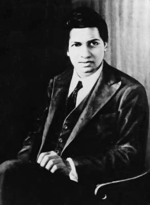
Ramanujan

If ever there were a mathematician par excellence, whose insights and discoveries are wrapped in inscrutable leaps of the imagination, it is Srinivasa Ramanujan. He is reputed to have said “An equation for me has no meaning unless it expresses a thought of God” [41]. He attributed his unproven mathematical results to divine intercession. He said that the Goddess Namagiri, his personal deity, “would write the equations on his tongue… [and] … bestow mathematical insights in his dreams” [41].

Among the countless formulae for \(\pi\) may be mentioned one, due to Ramanujan, which is so unusual that one wonders how it was ever derived in the first place: \[ \frac{1}{\pi} = \frac{\sqrt 8}{9801}\sum_{n = 0}^{\infty}% \frac{(4n)!\left[ 1103 + 26390n \right]}{(n!)^4 396^{4n}} \qquad{(22)}\] Was it another gift from the Goddess Namagiri?

Buffon’s Needle

In The Pi of Archimedes and this blog, we have seen the relationship between \(\pi\) and geometry and trigonometry. Such a relationship is not unexpected, for we may metaphorically say that \(\pi\) has its “home” in the circle, and is “neighbours with” trigonometric functions, which are also called circular functions. Even its link with infinite series may be justified as an extension of these relationships.

Interestingly though, \(\pi\) may also be estimated by repeatedly performing a random, or probabilistic, experiment, whose precise outcome cannot be predicted, but whose average behaviour may be estimated. But how indeed does \(\pi\) enter the domain of probability?

Georges-Louis Leclerc, Comte de Buffon was a French naturalist of the eighteenth century. Although his academic contributions were largely in the domain of the life sciences, he is today probably most well-remembered for proposing and solving a problem that goes by his name: Buffon’s needle problem.

There are several variants of Buffon’s needle experiment. The version we consider is to estimate how often a randomly thrown needle will intersect one of a series of parallel lines. In our variant, the needle is shorter than the perpendicular distance between the parallel lines. Interestingly, this experiment is a probabilistic method for determining the value of \(\pi\), and antedates modern Monte Carlo simulations on computers.

This experiment is one in which the precise outcome of any single throw cannot be predicted; but its average behaviour may be estimated with increasing confidence, as the number of throws increases.

Problem statement

The Buffon’s Needle problem may be posed thus. Consider a needle of length \(\lambda\)¹⁵ that is thrown at random on a floor that has parallel lines spaced \(d > \lambda\) apart [24].

What is the probability that the needle will touch or cross one of the lines?

We may assume that the needle’s position and its orientation, when it lands, are both independent and random.

Problem solution

This problem may be solved elegantly using trigonometry and the integral calculus. First we draw a diagram of how the needle may fall with respect to a pair of lines, as shown in Figure 10.

We have chosen the centre of the needle as the reference point or datum. It conveniently accounts for symmetry, as the needle could touch a line on either side of the centre.

In Figure 10, because the spacing between the parallel lines \(d\) is greater than the length of the needle \(\lambda\), we know that the needle can at most intersect one line of a pair. We have shown that pair of lines here. The perpendicular distance from the centre of the needle to the nearest parallel line is denoted by \(x\). By relating \(x\) to the angle \(\varphi\) and needle length \(\lambda\), we derive the condition for intersection or non-intersection as a simple inequality.

With reference to Figure 10, let \(x\) be the perpendicular distance from the centre of the needle to the nearest parallel line. If the needle makes an angle \(\varphi\) measured in the conventional sense with respect to the nearest line, the distance of the tip of the needle from the centre, in the direction perpendicular to the parallel lines, is \(\frac{1}{2}\lambda\sin\varphi\). Clearly, if \(x > \frac{1}{2}\lambda\sin\varphi\), the needle cannot touch the nearest line. Therefore the condition for the needle to touch the nearest line is: \[ x \leq \frac{1}{2}\lambda\sin\varphi \qquad{(23)}\]

Because of symmetry, we may restrict our consideration to angles \(0 \leq \varphi \leq \pi\) and for \(0 \leq x \leq \frac{d}{2}\). We may now define the event space as the rectangle on the \(\varphi-x\) plane bounded by the lines \(x=0\), \(\varphi = \pi\), \(x = \frac{d}{2}\) and \(\varphi = 0\), as shown in Figure 11. The event space represents all possibilities.

The set corresponding to the needle touching or crossing a line is the set of all points for which Equation 23 is satisfied. It is shown coloured in Figure 11.

In Figure 11, we have set \(3 = d > \lambda = 2\) without loss of generality in order to get a curve that can be plotted.

The orange area under the curve satisfies the inequality \(x \leq \frac{1}{2}\lambda\sin\varphi\). Its area is proportional to the totality of events where the needle touches a purple line. Let this area be called A. Then: \[ \begin{aligned} A &= \frac{\lambda}{2}\int_0^{\pi}\sin\varphi\;\mathrm{d}\varphi\\ &= \frac{\lambda}{2}\displaystyle\bigl[-\cos\varphi\bigr]_0^{\pi}\\ &= \frac{\lambda}{2}[-\cos(\pi) - (-\cos(0)]\\ &= \frac{\lambda}{2}\displaystyle\bigl[-(-1) -(-1)\bigr]\\ &= 2\frac{\lambda}{2}\\ &= \lambda \end{aligned} \qquad{(24)}\]

The greenish rectangle in Figure 11 represents the universal set of all events, or the event space, as noted before. It is bounded by the \(\varphi\) and \(x\) axes and the lines \(x =\frac{d}{2}\) and \(\varphi = \pi\) as shown. Its area is proportional to every throw of the needle in any experiment, and equals \(U = \frac{\pi d}{2}\).

The probability that the needle touches or crosses a parallel line is therefore equal to: \[ \begin{aligned} P(\lambda, d) &= \displaystyle\frac{A}{U} = \displaystyle \left[ \frac{A}{\frac{\pi d}{2}} \right] \\[0.5em] &= \displaystyle \left[ \frac{\lambda}{\frac{\pi d}{2}}\right ]\\[2em] &= \displaystyle \frac{2\lambda}{\pi d} \end{aligned} \qquad{(25)}\]

If a probabilistic experiment is repeated independently a great many times, the relative frequency of the event whose probability we are trying to measure, approaches the true probability. Using this principle, it is possible to simulate Buffon’s needle experiment on computer, calculate the relative frequency, associate it with the theoretical probability, and thereby evaluate \(\pi\).

Incidentally, the derivation of the probability \(P(\lambda, d)\) does involve geometry and trigonometry, and the appearance of \(\pi\) is not so inexplicable after all! 😉

Computer simulation

A Julia script that implements the mathematics derived above is available as buffon.jl. Note that because it is a simulation involving random numbers in Julia, any two consecutive results will not necessarily be the same. The estimated value of \(\pi\) can and does vary, quite significantly as successive trials are run. So, I am not documenting any results, but instead ask you to install Julia, execute the script by invoking julia buffon.jl, and inspect the results.

Abstraction

As explained above, it is important to realize that the analysis of the needle position with respect to a single line-pair suffices. This is an instance of problem abstraction or modelling, which is an important skill to acquire. It restricts focus to the essentials, and in the process usually simplifies the solution of the problem.

For a visual analogy, think of a surgical operation, where the patient is draped in green everywhere, except the site of the operation, and where the bright light is shone exclusively on that one area, so that the surgical team may concentrate on it without distraction.

The Brothers Chudnovsky

The Brothers Chudnovsky [42–44] embody in the popular imagination the archetypal digit hunters who are immersed in the quest for ever more digits of \(\pi\) [44–46]. Mark that we do not need \(\pi\) to two billion places for any earthly or unearthly¹⁶ purpose!

The Quest for Ever Greater Precision

In 1560, \(\pi\) was known only to 6 decimal places. By 1706, it had been computed to 100 decimal places. This jumped to 707 by 1874. In 1947, \(\pi\) was known to 808 decimal places. The advent of computers meant that by 1957, the number of decimal places had grown to 10,000. By 1967, this number had climbed up to 500,000. In 1997, researchers in Japan computed \(\pi\) to a mind-boggling 51.5 billion decimal places [47].

One may wonder what drives this quest for ever greater precision. As we have already observed, it is not driven by practical need. Hunting for ever more digits of \(\pi\) using ever more efficient algorithms that yield ever more decimal places has become a sport rather than a necessity.

Because \(\pi\) is ultimately unknowable as a decimal number, it has a mystery to it. Each successive attempt to improve the precision to which it is known, is a quest to tame the untameable.

But apart from aesthetic motives, the decimal expansion of \(\pi\) may reveal new knowledge about number sequences, randomness, and how to generate random numbers.

What mesmeric pull does \(\pi\) have on human imagination and endeavour to inspire such single-minded and unflagging pursuit? What is the magic within \(\pi\) that fuels such devotion and dedication? Is it beauty? Is it mystery? Or is it divinity?

Sources for Enrichment

If you are intrigued by the material in these two blogs on Pi¹⁷ and have the time and interest to find out more, do engage with some of these books, websites, and videos. They will enhance your knowledge of \(\pi\) and enrich you intellectually.

Book Recommendations

I recommend six books. The first is an encyclopaedic source book on \(\pi\) by Berggren et al. [32]. It contains a wealth of historical information and has facsimiles of many original publications or their translations. The second book follows on from the first. It chronicles the recent history of \(\pi\) and its computation [44].

Interestingly, the next two volumes are written by engineers, not mathematicians. Beckmann’s book [24], although somewhat dated and opinionated, is a labour of love. It gives detailed historical accounts of efforts at computing \(\pi\). The book by Banks[47] is a delightful, instructive and entertaining romp through some areas of applied mathematics. It is easy to read and devotes three chapters to famous numbers and number sequences.

Another interesting and accessible popular exposition, exclusively on \(\pi\), is the book by Posamentier and Lehmann [48]. Lastly, the popular book by Blatner [46] is historically informative and instructive.

Web Resources

If you are unsure about a mathematical term, or definition, I would recommend, as first port of call, Wolfram MathWorld, “created, developed, and nurtured” by Eric Weisstein [49]. It is a searchable, authoritative and encyclopaedic web site. Although Weisstein is himself an astronomer, his enduring love of Mathematics has resulted in this treasure trove of mathematical information on the web, from which all can benefit.

The lives of mathematicians have been chronicled at several places on the Web. One of the most comprehensive and scholarly—fully searchable, and with many related links—is the MacTutor History of Mathematics website [50].

You may find out more about the formulae for computing \(\pi\) at Pi Formulas. One particularly interesting formula is that of Wallis: it is composed of an infinite product of rational numbers to yield the irrational number \(\pi\).

If you wish to explore more about \(\pi\), the Fibonacci sequence, and other numbers, you may want to visit Ron Knott’s information-packed site.

One thread runs through this blog: mathematics is one interrelated structure in which the most unlikely connections between its disparate parts are a natural consequence of its inherent integrity. A delightful article on this idea, using Ramanujan’s work as its thematic centrepiece, is available online [51].

Media on the Web

How Augustin-Louis Cauchy solved the Basel Problem is clearly laid out and explained in this mesmerizing Rise to the Equation YouTube video [52]. The explanation in this video should be clear to a high school student who has encountered trigonometry but not calculus.

Those of you who are puzzled by the appearance of \(\pi^2\) in the solution to the Basel problem should also view this 3Blue1Brown YouTube vdeo [53].

Veritasium, Mathologer, and 3Blue1Brown put out quality educational videos on Mathematics on YouTube and are an authoritative source of enrichment. Do benefit from them.

An excellent biography of Carl Gauss is available on YouTube [31]. I highly recommend watching it.

A screen adaptation of Robert Kanigel’s biography of Ramanujan, The Man Who Knew Infinity [41], is also available. Watch it if you can.

There are two web sites with simulations of the Buffon’s Needle experiment. George Reese’s site has a discussion and simulation of the experiment. Michael Hurben’s site not only has a simulation, but also tracks and displays how close the estimate of \(\pi\) approaches the true value as the experiment is repeated.

Conclusion

We use pictures and words to communicate. In mathematics, geometry corresponds to pictures, and algebra to words. The interplay between geometry and algebra has been responsible for many mathematical advances. For example, the development of co-ordinate geometry laid the foundations for calculus and analysis.

Pi sits at the junction between pictures and words. It is geometrically defined, but its expression is algebraic. It is that ubiquitous magic number that shows up in the most expected and unexpected places. It appears in almost all areas of mathematics, including geometry, algebra, calculus, infinite series, and probability, to name a few. In our foray into \(\pi\), we have chanced upon two of the most important ideas in analysis: those of a limit and of convergence.

These blogs have chronicled the story of how \(\pi\) was extracted from the ore of geometry and refined into an enigmatic number which cannot be trapped within the confines of finite digits. It is a magnificent creature that forever eludes the implacable arrows of the digit hunters on their relentless quest for ever more digits of \(\pi\).

The history of \(\pi\) illustrates that mathematics is not merely a logical edifice built from the granite of unassailable logic. It is also the fruit of a pliant but disciplined imagination, fuelled by inspiration, that ever keeps expanding its boundaries.

Acknowledgements

I am grateful to my son, Mr Nandakumar Chandrasekhar, for writing the Julia script agm-float.jl to compute the AGM.

Free online computational support from Wolfram Alpha and ChatGPT are also gratefully acknowledged.

Feedback

Please email me your comments and corrections.

A PDF version of this article is available for download here:

References

•  pi (1)