Conceptual Abstract Algebra
2026-10-21 | 2026-11-18
Estimated Reading Time: 85 minutes
Abstract Algebra is a mathematical landscape that we encounter after we leave school. The warm familiar waters of solving equations give way to the forbidding, frigid ice-blocks of structural symmetry. It is as drastic a change as that which a baby faces on leaving the controlled environment of the womb to enter the unpredictable world outside. This shock must be mitigated by the books and people who are entrusted with managing this transition. Unfortunately, they mostly do not rise to the occasion. This short slog1 has been written to mitigate the shock of the transition and introduce the benefits of entering this new world. It relies on both words and pictures, and is targeted at the interested layperson.
Prelude
Imagine you are in front of a house in a residential neighbourhood. The houses are predictable, the environment clean, the silence resounding, and the peace tangible. It is as if the suburb had morphed into a neighbourhood of heaven.
You ring the doorbell in front of a house. When the door is opened, you are aghast to find inside the house a tropical rain forest with its varied vegetation and wild animals. A cacophony of strange and scary sights and sounds greets you.
Would you immediately run away, closing the door after you, or would you venture into the dark, dank depths of the uncharted forest inside?
Abstract Algebra, as a specialty of mathematics, has always seemed to me like that forbidding rain forest tucked away in a corner, behind the perfectly normal main doors of mathematics. One could live one’s entire life without venturing past that threshold. And millions do.
This blog was written to facilitate my entry into that rain forest, after the initial trepidation was overcome. And it is shared in the hope that it could help others take that momentous first step.
Music and Mathematics
Great music of any culture—Beethoven’s Ninth Symphony, or Michio Miyagi’s Haru no Umi, or Muthuswami Dikshitar’s Raṅgapura Vihāra—does not require expert musical knowledge to be appreciated. One only needs interest and a keen ear for melody and harmony, rhythm and beat, to enjoy these classics.
Likewise, to appreciate the beauty of mathematics one needs interest and an understanding of the logical principles and outcomes underlying mathematics. It should require no specialist preparation to be savoured and delighted in.
Alas that is not the case with contemporary mathematics. The maze of nomenclature, thickets of notation, and velvet curtains of symbols make natural appreciation all but impossible for the curious layperson. And I have always felt that the hoi polloi should not be fenced out by the literati.
The exquisite structures adorning the depths of mathematics are actually intricate masterpieces of beauty, no less than the greatest masterworks of art and music. Listening to great music should not require you to read musical notation. You only need interest and engagement. So too for mathematics.
It may be claimed that the innocent beauty of Creation itself is embedded in the warp and weft of mathematics. I have written this blog to de-mystify aspects of abstract algebra for myself. If, when they are shared, they can do something similar for my readers, I would be deeply fulfilled.
Mathematics is self-regulating
Historically, mathematics has been marvellously self-regulated by her practitioners. Witness the revolution in arithmetic occasioned by the use of Hindu-Arabic numerals to replace Roman numbers. But sometimes, the practitioners race so far ahead that the general public gives up, as futile, the pursuit to keep up with changes. Abstract Algebra is one such runaway stallion.
Fun YT Video to watch first
If you can spare twenty minutes to watch a YouTube video, I will recommend this whimsical romp through the realm of mathematics created by Martin Kuppe, aka Zogg from Betelgeuse. In it, at around 11:30 there is an attractive map of a place playfully called “Mathematistan” [1].
In everyday life, we have nouns and verbs, names and actions, words and pictures. We will strive to look at these twin aspects as we survey the vast domain of mathematics.
Sets
Although Sets are strictly not algebraic structures, they are the underlying base for all of them. Think of Sets as the roads on which the vehicles called Algebraic Structures run. A set is simply a collection of “somethings” bound by a description. They obey logical operations, like “a double negative is a positive,” but possess no inherent arithmetic machinery like the number systems. We take a look at a simple example below.
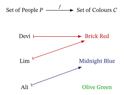
Sets allow us to define a mapping from the elements of one set to the elements of another, or back into the same set itself. Suppose we have a set of three people and a set of available colours, and we want to map each person to their favourite colour. Figure 1 illustrates one such possible mapping. Note the following points:
Every person is mapped to exactly one colour. This is the strict definition of a function.
Two people may be mapped to the same colour. A function does not have to be one-to-one, or injective.
Some colours might have no one mapped to them. A function does not have to be onto, or surjective.
From water to algebraic structures
Numbers and arithmetic are familiar to everyone. Calculus, differentiation, and integration are known to the high school student. Vector spaces and fields are the bread and butter of engineering students at university. We will now classify some structures in mathematics by the rigidity imposed on what they can and cannot do. What do I mean by a hierarchy of constraints that impose rigidity?
Let us use water as an example. As water vapour, it is hardly seen. It does not have dimensions, shape, etc. As a gas, it does not even have a direction of flow unless there is a wind. It simply diffuses. Water vapour resembles the elements of a set in set theory.
When the water condenses, it might become a river with a clear direction of flow. But shape and dimensions are still elusive. Pour the water into a pitcher, and it assumes the shape of the pitcher. The volume may be measured. Liquid water is a metaphor for a group.
Freeze the water in a container. The water becomes frigid and rigid. Its dimensions may be measured. It resembles a vector space. Short of melting it, the freedoms enjoyed by water in its liquid and gaseous states elude it when it is solid.
The Nouns and Verbs of Abstract Algebra
In everyday life, we use nouns to identify objects and verbs to denote actions. The same dichotomy applies to the denizens of Abstract Algebra. The emphasis to keep in mind is that:
Verbs dominate Nouns in Abstract Algebra.
Nouns: Elements, Sets, and Spaces
The nouns are called Elements, Sets, or Spaces, depending on context. When we talk of actions on individual members of a set, we call them Elements. The arena where these actions take place is called either a Set or a Space.
Verbs: Operations, Mappings, Functions, or Homomorphisms
When an action takes place within the same Set, we call it an operation. An example is the combining of two numbers through addition to give a third number in the same set.
When the action takes place across different Sets, we call them Mappings, Functions, or Homomorphisms. These translate the rules of one space into another. An example is shown pictorially in Figure 1.
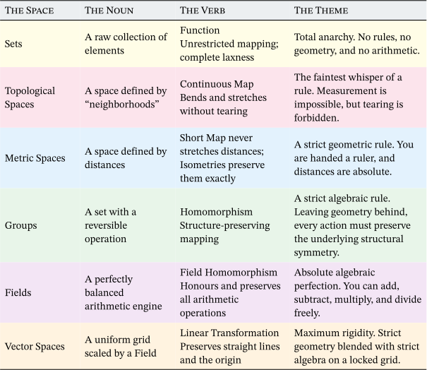
Several mathematical spaces, their nouns, verbs, and the constraints that are imposed on them, along with their resulting properties are summarized in Figure 2.2 Sets, fields, and vector spaces are likely to be more familiar than the others. This table is indicative rather than comprehensive and the purpose has been to illustrate the richness that results from following the discipline imposed on each category or space.
Escalation of Rigidity
What do we mean by “escalation of rigidity”? Suppose that we stack algebraic structures that obey fewer rules at the bottom, and keep on adding one rule and one structure at a time to the top. We will be building a pyramid where the structures lower down have more fluid behaviour while those higher up exhibit more constrained or disciplined behaviour. I call this the “natural stacking order” of algebraic structures. The behaviour becomes more rigid as we ascend the pyramid. This is escalation of rigidity.
The “natural stacking order” of algebraic structures has the admirable property that the more rigid structures embody all the properties of the less rigid structures beneath them in the pyramid.
Groups
Although we are discussing Groups right after Sets, they are not on the next rung in the ladder of escalating constraints. Two other structures, called Semigroups and Monoids, intervene.3
Groups share the properties of Sets, Semigroups, and Monoids, all of which are foundational in the same sense as the foundation of a building. But Groups also embody an Inverse operation.
The inverse operation uniquely distinguishes a Group from the weaker structures beneath it.
Verbs are more central to Groups than Nouns. Let \(f\) be an action that does something in a Group. The ability to undo means that we must have another action, let us say \(g\), such that applying \(f\) and then \(g\) restores the element to its original state. We call \(g\) the inverse of \(f\).
This internal ability, via the inverse, to undo what has been done is the primary characteristic of a Group. The consequence of this strict constraint is that we must always be able to return to our starting state. Inverses are internal to a Group.
But this rigidity yields a spectacular secondary benefit that allows us to bridge Groups conceptually. We are now able to compare two different Groups systematically. When we find a perfect, “structure-preserving mapping” between two different groups, we call it an isomorphism.
An inverse is an internal action that operates within a single Group, whereas an isomorphism is an external mapping that translates across two different Groups.
Consider a collection of four numbers with multiplication, and a four-sided figure with equal sides—namely a square—undergoing rotations of 90°. Placing these two operations side-by-side, as in Figure 3, we clearly see that although we are dealing with multiplication by numbers on the one hand, and rotations of a geometric figure on the other, the similarity between the two operations are apparent even to the untutored eye.4
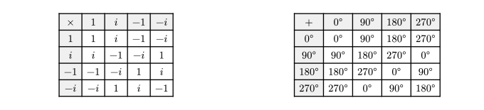
What we have done is to abstract or “draw out” the essence of two different operations and display the resulting similarity for all to see. Like an ultraviolet light can display characters written in invisible fluorescent ink on a piece of paper, Group Theory makes obvious those patterns that might otherwise escape detection.
At school, you might have heard of bijections, or one-one and onto mappings. An isomorphism is a bijective mapping between two structures that preserves the underlying operations or relations.
Isomorphisms act like mirrors. They allow us to share the solutions to already solved problems with new or difficult problems, so long as an isomorphism has been identified between the two. The ready solution may then be applied to solve the new or difficult problem. This accelerates the development of mathematics as a whole, and also better integrates the various branches in it.5
Compositions
Consider compositions in Group Theory. Let us start with an example. Consider these equations: \[\begin{aligned} 2 + 3 &= 5\\ 10^{(2 + 3)} &= 10^5\\ 10^2 \times 10^3 &= 10^5 \end{aligned}\qquad{(1)}\]
What do these equations tell us? If we take a pair of numbers, and add them, and then using \(10\) as base, exponentiate using the sum, we will get the same result as if we applied each number in the pair as an exponent to \(10\) and multiplied the result. This much is known from the logarithms encountered in school algebra.
This equivalence is schematically shown in Figure 4 below, illustrating the fundamental exponential law \(10^{a+b} = 10^a \times 10^b\).
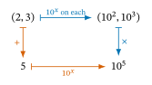
It is a concrete example of a group isomorphism—a structure-preserving translation between two distinct arithmetic systems: addition of real numbers and multiplication of positive real numbers.6
Group Theory cares about the internal algebra. It looks at the elements—like \(2\), \(3\), and \(5\)—and verifies that the rule \(10^x\) perfectly maps the addition of the first system to the multiplication of the second. It focuses on the specific behaviour of the elements and operations to prove that an isomorphism7 exists. Group Theory guarantees that the numbers behave properly.
Practical Applications
Groups might seem like an abstract idea suited to pure mathematics, but with little real-world application. And in this, you would be grossly mistaken. Groups are constrained by fewer rules than, say the very numbers we use. And because of this, they appear in all sorts of places as abstractions of structures.
Particle Physics
In the prevailing paradigm, fundamental particles are not just tiny spheres; they are classified by their symmetries. The symmetry group of the Standard Model of particle physics is the combined group \(SU(3)\times SU(2)\times U(1)\). Particles fall into families that correspond to the ways a group can act, and a gap in a family is a prediction.
The most celebrated case: in 1962 Murray Gell-Mann used the pattern of a related symmetry group, also called \(SU(3)\), to predict a missing particle, the \(\Omega^-\), which was found in 1964. That is how tangible—and paradoxically intangible—something abstract has become!
Cryptography
Much of the cryptography that protects bank transfers and encrypted websites is built on finite groups. The Diffie-Hellman key exchange, and its elliptic-curve cousins, live in a finite cyclic group: pick an element \(g\) and keep multiplying it by itself. Repeating the action \(a\) times, to get \(g^a\), is quick. But recovering \(a\) from the outcome \(g^a\) (the “discrete logarithm”) is believed to be hopelessly slow in well-chosen groups.
The RSA algorithm works in a different finite group: the invertible whole numbers modulo \(n = pq\), where \(p\) and \(q\) are two large primes. This group is not cyclic, and its security rests on a different difficulty, that of factoring \(n\) without knowing \(p\) and \(q\). Is it not a measure of the power of Groups that the simple qualitative explanations thus far have made cryptography comprehensible?
The Essence of Groups
It has been observed that “Numbers measure size, groups measure symmetry.” [2]. Whether we are rotating a physical square, multiplying by imaginary numbers, or tracking the spin of a subatomic particle, we are studying the same phenomenon: the ability to change a system while leaving its essential core completely unchanged. Group Theory is the universal language of that preservation. It teaches us that symmetry is not just a visual property of butterfly wings and snowflakes; it is a rigid, underlying structural law of the universe.
We have now come to the end of our cursory introduction to groups. If you would like to probe further, I would suggest the reader-friendly books by Pinter [3] and Carter [4]. A curated list of books is also offered as suggestions for further reading at the end of the blog.
Fields
The word field is well known from its use to describe regions of space in which certain forces are experienced. Gravitational, magnetic, and electric fields are familiar examples. But the word as it is used in mathematics carries a totally different meaning.
A field is an arena in which arithmetic may be performed. Think of it as resembling a tennis court on which tennis may be played. And why do we dignify it with a dedicated name? Because fields are vital to mathematics. And because the family of fields is extensible without bound.
If a group represents the strict enforcement of the single rule of reversibility, a field represents absolute algebraic perfection. I touched upon fields in a previous blog when discussing the Fundamental Theorem of Algebra. There, it was stated that a field is a set of numbers, closed under all four basic arithmetic operations: addition, subtraction, multiplication, and division.
But how does a field fit into our hierarchy? A field represents the progressive evolution of a group. It is in fact the child of two groups: an additive Abelian group8 that allows us to add and subtract, and a multiplicative Abelian group—excluding zero—that allows us to multiply and divide. It shares the same space as its two parent groups.
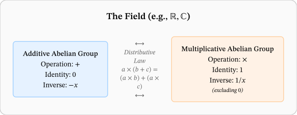
What happens when we “cross” these two groups? How do we derive a field? The properties of an additive group and a multiplicative group in isolation are shown in the coloured boxes in Figure 5.
But if they were simply boxed together, there would be no benefit. They could as well have remained separate. To allow the two groups to “communicate” we need to link them with a special “chromosome”, or “umbilical cord”, or mathematical bridge that lays out how addition and multiplication should interact to give us a consistent arithmetic.
And that is the distributive law of multiplication over addition, shown at the centre of Figure 5. This vital link breathes life into a field. The resulting happy hybrid is called a field and is fully empowered to do all of arithmetic.
Thus far, we have only concentrated on the operations or morphisms that a field is capable of. But what about the associated sets? Only certain sets of numbers qualify to be fields because they must be closed under the arithmetic operations. Examples include the rational numbers, \(\mathbb{Q}\), the real numbers, \(\mathbb{R}\), and the complex numbers, \(\mathbb{C}\). Are there other fields? By Jove, yes.9
Fields are like dance partners to vector spaces. We cannot have a vector space without naming its corresponding field. They always occur in pairs. And it is vector spaces that we turn our attention to next.
Vector Spaces
Vector Spaces are where vectors live. Vectors are pointy arrows with an attached stem. They are connected head-to-tail when added, according to the parallelogram law. They can be stretched by multiplication by a factor, say \(k\). This scalar, \(k\), is supplied by the field \(F\) associated with the vector space. These are the possibilities:
If \(k < 0\), the direction of the vector is reversed.
If \(\lvert k \lvert \in (0, 1)\), the size of the vector is reduced.
If \(\lvert k \lvert \in (1, \infty)\), the size of the vector is increased.
If \(k = 1\) the vector remains unchanged.
If \(k = 0\) the vector disappears.
This much should be familiar from high school physics. But is this all there is to vector spaces? Why should they be accorded their own space?
Mathematicians abstracted from vectors their fundamental characteristics of addition with each other and multiplication by a factor. Needless to say, as in all algebraic structures, these operations are closed. They then found out that not only the vectors of high school, but many other mathematical objects also possessed “vectorial” characteristics. And this led to the grand generalization of the idea of a vector into that of a vector space.
Because vectors can be added, a vector space must define and enable addition of its elements. Because vectors can be scaled, there must be some number that can be applied to vectors to enlarge or diminish their magnitudes. This realization has two consequences:
Every vector space must be paired with a field that will supply the numbers to scale the vectors.
Addition of elements of a vector space must mirror the addition of vectors as known in high school.
Let us keep amorphous exactly what lives in a vector space. Even so, we can definitely deal with two entities: vectors, and scalars which are numbers.
A vector space comes with exactly two internal operations of its own: adding vectors together, and scaling a vector by a scalar from the field \(F\). These must obey a short list of strict rules:
The vectors form an Abelian group under addition;10
Scaling distributes over vector addition: \(k(\mathbf{u} + \mathbf{v}) = k\mathbf{u} + k\mathbf{v}\);
Scaling distributes over scalar addition: \((k + l)\mathbf{u} = k\mathbf{u} + l\mathbf{u}\);
Scaling is compatible with multiplication in \(F\): \((kl)\mathbf{u} = k(l\mathbf{u})\); and
\(1\mathbf{u} = \mathbf{u}\).11
When we map one vector space to another, the mappings worth studying are those that perfectly respect these two internal operations. For historical reasons, these functions are given the moniker \(T\), for transformation, rather than the usual \(f\). Vectors are usually denoted by bold symbols and scalars by italic letters. The defining rules become: \[\begin{aligned} T(\mathbf{u} + \mathbf{v}) &= T(\mathbf{u}) + T(\mathbf{v})\\ T(k\mathbf{u}) &= kT(\mathbf{u}). \end{aligned}\qquad{(2)}\]
This pair of equations defines a linear transformation: a map between vector spaces that respects their internal addition and scaling.
Let us shine a bit more light on Equation 2. Let \(T\) be a map from \(V\) to \(W\), both being vector spaces. Let \(\mathbf{u}\), \(\mathbf{v}\), and \(\mathbf{w} = \mathbf{u} + \mathbf{v}\) all be members of \(V\). Closure of operations in \(V\) guarantees that \(\mathbf{u}\), \(\mathbf{v}\), and \(\mathbf{w}\) are all members of \(V\).
Likewise, closure of operations in \(W\) guarantees that \(T(\mathbf{u})\), \(T(\mathbf{v})\), and \(T(\mathbf{w})\), are all in \(W\). Moreover, the linearity from the sum is also preserved.
If you stop to think about it, this is a strong constraint we are applying on \(V\), \(W\), and \(T\). The same comments apply to the scaling part of the definition of \(T\). The fact that Equation 2 at all holds means we are likely to reap rich dividends from this setup and, indeed, we do.
Anatomy of a Vector Space
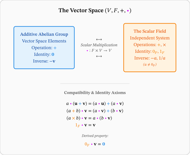
In Figure 5, we looked at the innards of how a Field is assembled. This is the right juncture to do the same for a Vector Space. By viewing Figure 6 in conjunction with Figure 5, let us imbibe the profound lessons in frugality that Abstract Algebra has to offer us.
Frugality and Re-purposing
A Field is the fusion of two Abelian groups connected by the distributive law. A Vector Space is again the fusion of two abstract structures: an Abelian group and a Field, linked this time by the operation of scalar multiplication.
After a field has been constructed (as in Figure 5), it is available to be used on its own as an independent component in the definition of another structure. Just as motorcar components like alternators or brake calipers can be re-used across entirely different vehicles, mathematical components can be re-used to build new spaces. This “building upon the already built” is emblematic of the frugality of mathematics.
Notice that the Field and the Vector Space both feature an Additive Abelian Group (AAG). Both have three operations—addition, an identity element, and an inverse element—that are highlighted in their respective diagrams.12 It may be argued that the left-hand AAG in Figure 6 is structurally the same group as that on the left of Figure 5.
The verbs (the operations) are identical. Only the nouns have changed.
The AAG of a Field uses the addition of numbers. The AAG has simply been re-purposed in a Vector Space to handle the addition of vectors. The descriptive text “Vector Space Elements” has been added in Figure 6 only to clarify the nouns associated with this specific arena.
The rather confining straitjacket of algebraic axioms becomes necessary precisely because we want to enjoy this convenience of re-purposing. By not naming the objects—but rather defining the guardrails of how they act—we ensure the mathematics does not go astray. This same idea resurfaces as polymorphism in programming languages.
Colour-Coding the Operations
Because we are re-using verbs across different nouns, we must be careful not to blindly extrapolate the careless arithmetic of high school. In Figure 6, the operations have been carefully colour-coded to ensure we know which operation belongs to which domain.
The AAG and its vector elements are in blue. The Field and its scalar elements are in orange. The sole operation connecting the two spaces is scalar multiplication, denoted as a centred pink dot (\(\mathbin{\color{magenta}\bullet}\)).
This colour coding sheds light on how each small step in a chain must be a valid operation consistent with the underlying structure. Note especially that scalar multiplication maps an ordered pair (a scalar from the field and a vector from the AAG) into a resultant vector back in the AAG. Symbolically, this is denoted as \(\mathbin{\color{magenta}\bullet}: F \times V \to V\). The left and right plus signs, and the dot, all have strict, non-interchangeable meanings. The sequence of axiom stacking is designed so that every new rule is completely supported by the frugal foundation beneath it.
Because we now understand the internal mechanics of a Vector Space—just as a master mechanic understands an engine—we are free to swap the components. For example, we can marry the set of polynomials of degree up to two, \(P_2\), with the rational field \(\mathbb{Q}\). As long as this new pairing obeys the frugal rules of the Additive Abelian Group and scalar multiplication, we have successfully created a brand-new Vector Space, ready to be explored for its unique properties and utility.
Building plan versus bricks and mortar
I want to digress briefly to introduce a metaphor about vector spaces. Apart from the rules of arithmetic encapsulated in the field \(F\) associated with a vector space, we have a set of different rules relating to vector addition. Vectors cannot, in general be multiplied. So, scalar multiplication governs the aspect of multiplication in a vector space.
We have said a fair bit about vectors, but have we pinned them down to any one instantiation, any one embodiment? If you read carefully, you will notice that we have not particularized the vectors, we have only characterized them. Vector spaces are amorphous to us as far as their contents are concerned.
Herein lies the breathtaking austerity of the linear transformation, \(T\). It demands so little—merely that addition and scalar multiplication are respected—yet it delivers so much. Because we have strictly enforced these two rules while keeping the actual contents of the space amorphous, we are no longer restricted to vectors as lines with pointy arrows drawn on paper.
Anything that obeys these two austere rules is legally a vector. A polynomial like \(3x^2 + 2x + 1\) can be added to another polynomial and scaled by a number; therefore, polynomials are vectors. A matrix, which is a grid of numbers, can be added and scaled; therefore, matrices are vectors. As we will see later, when we explore Inner Product Spaces, even continuous waves of sound can be treated as vectors.13
It is this abstraction that gives vector spaces their staying power. They exist because they are useful. They are useful because they are powerful. They are powerful because the paradigm of vectors in vector spaces can be applied to very many real-life situations with exact concordance. We will see later some “far out” applications of vector spaces. For now, let us get back to the analogy.
Before a building is built, the architect and structural engineer will prepare plans that specify the way the building divides up space to perform its functions. But space cannot be divided without bricks and mortar, or plywood and drywalls. The building plan prepared by the draughtsman is the abstract vector space. The actual nuts and bolts, steel beams and floor slabs, bricks and mortar is the manifestation of the plan. The two are linked, one being a material realization of the other. They are in total harmony. But they are not the same.
That same plan could be used to build a hundred apartments or houses, but they are different concretizations of the same plan. They are alike but not identical.
Something like this happens when we particularize a vector space by superimposing conditions on the space. Mind you these superimpositions do not alter even one jot the structure of the vector space. They are simply external appearances of the same idea. Like the fins and tail on a fish happen to aid it in swimming in water, so do our legs enable locomotion on earth.
One such grid or superimposition is to treat vectors as ordered pairs of numbers. The complex numbers may be viewed as 2D numbers. The three-dimensional Euclidean space, denoted by \(\mathbb{R^3}\) may be associated with a triplet of numbers denoting a point in space with respect to a particular origin.
Note that all these are vectors, but the vector space does not worry about dimensionality or origin or any of the minutiae involved in particularizing a vector space. These attributes do not belong to the essence of a vector space. By abstracting the essentials from the vast multiplicity of its manifestations, we have a very concentrated “Essence of Vectors” that can be put to use anywhere vectors find application. Think of it as a juice concentrate that can be diluted for use.
This is the real reason why Abstract Algebra arose: to abstract the common structural patterns underlying diverse mathematical systems.
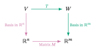
The abstract vector space-to-vector space transformation gets particularized once we associate \(V\) with \(\mathbb{R}^n\) and \(W\) with \(\mathbb{R}^m\). The transformation \(T\) takes on the garb of the matrix \(M\). It does not matter how we get from the top left corner to the bottom right corner. We can travel across-and-down or down-and-across. The destination is the same.
Another subtlety is hidden in Figure 8. The upper left-to-right arrow, \(V \to W\), links the coordinate-free world of pure geometry. No axes exist there. The lower left-to-right arrow, \(\mathbb{R}^n \to \mathbb{R}^m\) is in the co-ordinate world of Descartes where geometry is clad with the heavy numerical machinery of arithmetic and algebra. The two top-to-bottom lines bridge the abstract and the concrete. The burden of the abstract transformation \(T\) can now be assumed by the matrix \(M\), which is capable of the heavy lifting required in the real world. We can think geometrically, but compute algebraically, without losing the truth. This connection between geometry and algebra is a recurring and powerful leitmotif in much of mathematics.
Geometry is the vision. Algebra is the materialization.
Matryoshka Dolls: A versatile metaphor
I would like to digress briefly to describe a visual analogy that will prove useful henceforth.
Nested Russian dolls or Matryoshka dolls are apt metaphors in many mathematical settings. I have used the idea once before in another blog to help explain a nested sequence of intervals in analysis.
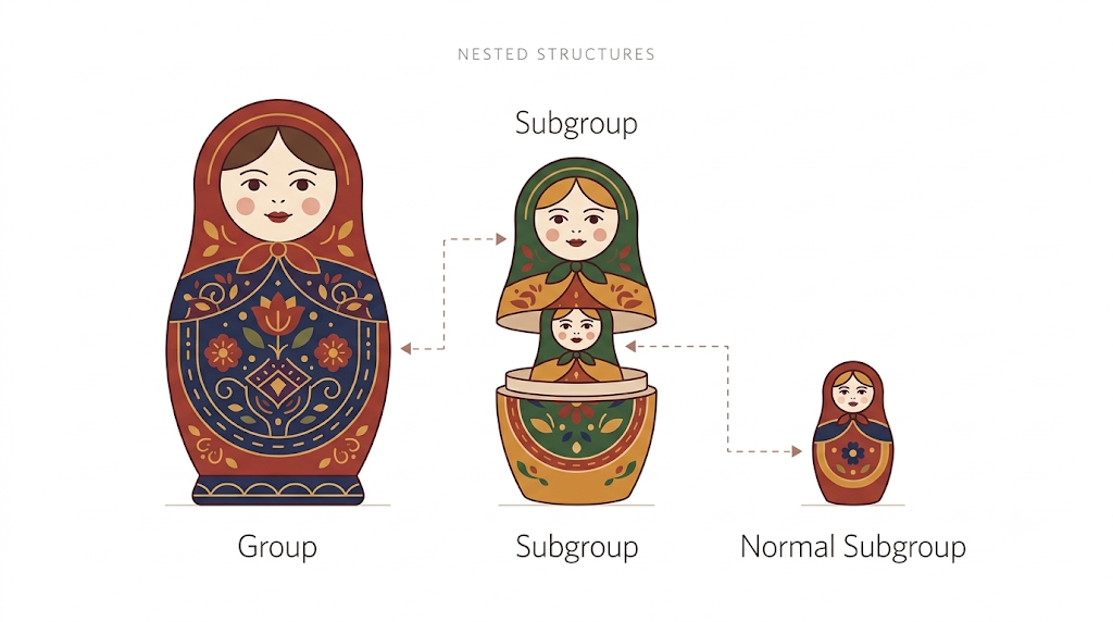
A schematic of nested Matryoshka dolls is shown in Figure 9. The dolls are graded in size and stacked one into another, with the inner dolls being smaller in size than the outer ones. The innermost doll represents the smallest possible size.
This much is always true of the metaphor conveyed by Matryoshka dolls. In the context of abstract algebra, the dolls may serve two different purposes. They may be harnessed to exemplify either the properties within a single algebraic structure or the properties across different algebraic structures.
Intra-structural nesting
This means that all the dolls are representatives of the same algebraic structure. If the dolls represent sets, the properties of all the dolls are the properties of sets. The difference is one of size, not kind.
The smaller inner dolls are obviously subsets of the outer ones, and the innermost doll is the smallest, ultimate subset. It is the empty set, \(\emptyset\), which contains nothing at all. It is, however, a subset of every set. Like the zero in our number systems, “The Nothing that Is” has been dignified by a name, signifying its importance.14
What happens when nesting is applied to Groups? Just as sets may contain subsets, groups may contain subgroups. These nested subgroups are groups in the their own right, and they share the same operations as the parent group. The deeper the nesting, the smaller the size of the group. And every subgroup perforce contains the identity element.
In this schema, the innermost doll represents the smallest irreducible group in this family that can still be called a group. It results from whittling down the valid actions of the group, shedding elements layer by layer, until only the solitary “do nothing” identity action survives. This doll represents the trivial group which consists of only the identity element, \(\{e\}\). There is a certain austere starkness as one moves from the outer dolls to the inner ones.
If the algebraic structure is a vector space with its associated field, the innermost doll would contain the zero subspace \(\{\mathbf{0}\}\).15
On a philosophical note, when we traverse the nested sequence of dolls representing any single algebraic structure, we move from the well-populated outer dolls to the innermost one which has but a single element. And that element is the analogue of the idea of zero or one, as it is represented within the conceptual framework of that specific algebraic structure.
Trans-structural nesting
From the second viewpoint, each doll represents a different algebraic structure. The difference between successive dolls is both of size and kind. Size may be taken as the numerical abundance of any structure compared to other algebraic structures in the structural universe. Kind is denoted by the axioms that characterize any particular algebraic structure.
When we traverse the spectrum from a formless Magma,16 to a Group, to a Ring, and finally to a Field, we are looking at a nesting that embodies a hierarchy of increasing constraints, coupled with decreasing numerical abundance in the universe of algebraic structures.
That was a mouthful. What exactly does it mean? As we impose more rules, demand more symmetries, and seek more profound patterns, we reduce the pore size of the mathematical sieve that allows the passage of qualifying structures. Fewer structures can pass through. And that in turn reduces the relative abundance of the more constrained structures. There are infinitely more formless Magmas in existence than there are highly-disciplined Fields.
In mathematics, formidable structural rigidity comes at the cost of insular exclusivity.
The Implicit Rules of the Matryoshka Dolls
While Matryoshka dolls are a useful mathematical metaphor, viewing them correctly requires understanding one implicit rule of the taxonomy of abstract algebra:
Axioms dictate what a structure demands, not what it forbids. They are floors, not ceilings.
Accordingly, mathematicians classify objects by the tightest, most specialized set of rules they obey—their maximal structure.
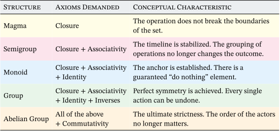
For example, a Magma is a set with one criterion: closure.17 No other criterion is demanded of a Magma.
A highly complex structure, like a Group, satisfies by default the singular rule of closure that characterizes a Magma, as it is “sitting inside” the larger Magma doll. But a Group is also very much more than a Magma. The Matryoshka dolls define the strict version of each structure—representing objects that meet a specific set of demands, but fail to qualify for anything higher.
The moment a structure reliably obeys a new rule, it is promoted. As we will see, if a basic Magma suddenly guarantees associativity, it is instantly reclassified as our next doll: the Semigroup. Thus, the logic and the nomenclature of the hierarchy are kept rigorous, taut, and consistent.
Although it puts us a little ahead of our narrative in the blog, the “escalation ladder of axioms” that is used for tightening successive algebraic structures is shown in Figure 10.
Intermezzo: Abelian Groups and Inner Product Spaces
We will now take two short pauses in our journey to consider Abelian Groups and Inner Product Spaces, each of which holds its own place of pride in the hierarchy of algebraic structures. An analogy about how these structures evolved historically will help.
Different types of roads
Consider different types of roads. It could be a rural dirt road, a narrow village road just wide enough for two-way traffic, a city road with zebra-crossings, traffic lights, and pavements, or an eight-lane high speed expressway designed for heavy nonstop traffic travelling cross-country. All roads are meant to carry vehicles, but restrictions apply according to type and use. The highway code applies to each, but with variations suited to place, purpose, and usage.
Algebraic structures are like this. The basic ones enforce the least number of constraints because they derive their power and generality from their frugal rules. Specialized ones are built later to serve explicit needs. That is the case with Abelian Groups vis-a-vis Groups, and Inner Product Spaces vis-a-vis Vector Spaces.
Groups and Abelian Groups
Groups were born from the tormented mind of Évariste Galois,18 who was perhaps one of the few mathematical revolutionaries who was also a political one. Let us cast our minds back on the groups Galois fathered.
To take the discourse on Groups one notch up the ladder of mathematical precision, let \(G\) be the set and \(\ast\) be the operation defined on it. Let \(f\), \(g\), \(h\) be elements in the group. Moreover, let \(e\) be the identity element, and let the inverse of \(f\) be denoted by \(f^{-1}\). The axioms governing Groups are four in number:
Closure: \((f \ast g) \in G \;\forall\, f, g \in G\)
Associativity: \((f \ast g) \ast h = f * (g \ast h) \;\forall\, f, g, h \in G\)
Identity element: \(f \ast e = e \ast f = f \;\forall\, f \in G\)
Inverse element: \(f \ast f^{-1} = f^{-1} \ast f = e \;\forall\, f \in G\)
But wait! What happened to the ability to swap the order of operations? Where is \(f \ast g = g \ast f\)? It has sneaked into the last two axioms, but they are special cases where the inverse and identity operations require the result to be independent of the order of the operands. But these are special cases and definitions, not general statements.
Indeed \(f \ast g = g \ast f\) is not a group axiom. But what about the additive and multiplicative groups? They only enforce associativity, which allows a binary operation to be chained indefinitely. But there is simply no rule to enforce, say, \(a + b = b + a\), or \(ab = ba\). If you are shocked, you have a right to be.
In school, our first encounters with arithmetic were with the addition of numbers or the memorization of multiplication tables. These emphasize commutativity: \(5 \times 2 = 2 \times 5 = 10\). The order of the operands may be swapped to give the same result. Unfortunately, this rule was not basic enough for commutativity to join the high table of the list of axioms for groups. Commutativity is not a universal rule of Nature—it is an incredibly rare, fragile exception, with extremely powerful consequences.19
The mathematical property of commutativity, in this context, was pioneered by Niels Henrik Abel as he investigated the symmetries of polynomial roots. The formal structure of what we now call a Group was introduced slightly later by Évariste Galois. Both men tragically died young, before their work could be fully merged. It was only decades later that the term Abelian group was applied posthumously to honour Abel’s pioneering work with commutative structures.
In the evolution of mathematics, the frugality of axioms seems to be a fundamental determinant in identifying algebraic structures. Throw almost everything away, and see if what remains can be of use.
Why are Abelian groups so important? The blasé answer is that they are powerful and useful. The observant among you would have noticed that I sneaked in the adjective “Abelian” in front of the additive and multiplicative groups in Figure 5, without explanation. Pardon me for that omission. It will now be redressed.
A group becomes Abelian with the addition of a fifth axiom:20
- Commutativity: \(f \ast g = g \ast f \;\forall\, f, g \in G\)
Commutativity guarantees sequence independence: the final mathematical state is completely immune to the chronological order of operations.
Applications of Abelian Groups
Abelian groups find widespread mathematical application in contemporary mathematics. Three of these are outlined below.
The Foundation of Vector Spaces
Abelian groups are an indispensable prerequisite for Vector Spaces. To add vectors using the parallelogram law,21 the order of addition cannot matter. Moreover, the geometric grid must be respected.
If we walk 3 blocks East and 4 blocks North, we must arrive at the same destination as walking 4 blocks North and 3 blocks East. If vector addition were not Abelian, physical space would warp depending on the sequence of your steps, and the parallelogram law itself would fail. Commutativity for addition is not a luxury but a necessity in our physical world. It might even be called an attribute of space.
The Engine of Fields
Standard arithmetic takes place in fields. From Figure 5 a Field requires two Abelian groups—one for addition, one for multiplication. If you strip commutativity away, you lose standard arithmetic entirely. You would end up in the bizarre realm of matrices or quaternions, where \(A \times B\) does not equal \(B \times A\). Abelian groups are the only reason we can compute balance sheets, or do high school algebra. Moreover, they offer the reassurance that our earliest encounters with arithmetic were neither untrue nor in vain.
The Privacy Shield of the Internet
Every secure transaction on the Internet—banking, WhatsApp messaging, email—relies on Public Key Cryptography, examples of which are Diffie-Hellman or RSA.
Here is the idea behind Diffie-Hellman. In a finite cyclic group with a public element \(g\), Alice secretly picks a number \(a\) and publishes \(g^a\); Bob secretly picks \(b\) and publishes \(g^b\). Alice raises Bob’s published value to her secret power, and Bob raises Alice’s to his: \[(g^b)^a = g^{ba} = g^{ab} = (g^a)^b.\] Both arrive at the same shared key, \(g^{ab}\), while an eavesdropper who sees only \(g^a\) and \(g^b\) is believed unable to compute it. The middle equality is commutativity at work: the exponents multiply in either order, so the two parties can apply their secrets independently, at different times, and still agree. Strictly, all that is needed is that powers of a single element commute with each other, which is true in any group.
Inner Product Spaces
If the signature characteristic of Abelian groups is sequence-independence arising from commutativity, the defining trait of Inner Product Spaces is the ability to measure sameness and magnitude.
A bare vector space is austere. We can add and stretch vectors, but the space itself is geometrically blind. It has no concept of length or angle. To equip the space with a ruler and a protractor, we must introduce the inner product—an operation designed to measure the “degree of sameness”, or overlap, between two vectors.
But before we can measure this overlap, we must resolve a fundamental problem regarding magnitude.
Measuring a vector against itself should logically yield its magnitude, or squared length. In the physical world, length is a strictly positive quantity. Even to use concepts like “positive” or “greater than zero,” our underlying arithmetic must happen in an ordered field—a field with a built-in sense of \(<\), \(=\), and \(>\).
The real numbers \(\mathbb{R}\) form an ordered field, allowing us to naturally speak of one number being greater than another. But Vector Spaces often operate over the complex numbers \(\mathbb{C}\), which have no built-in sense of order. In the complex plane, asking whether \(3i\) is greater than \(2 + i\) is mathematical nonsense.
So, how do we extract a strictly real, positive magnitude from a complex vector? We require a mathematical operation that always lands us back in the ordered realm of the non-negative real numbers.
We use the complex conjugate. The algebraic operation of multiplying a complex number \(z\) by its conjugate \(\overline{z}\) acts as a predictable map from \(\mathbb{C}\) down to \(\mathbb{R}\).22 The product \(z\overline{z}\) is mathematically guaranteed to yield a positive real number. To see how, let \(z = a + bi\) and \(\overline{z} = a - bi\). Then, \[\begin{aligned} z\overline{z} &= (a + bi)(a - bi)\\ &= a^2 - abi + abi -(bi)^2\\ &= a^2 + b^2. \end{aligned}\qquad{(3)}\]
Rather than creating one set of rules for real numbers and a different, patched set of rules for complex numbers, mathematics uses a single, unified definition. We start in the complex field and build the conjugate directly into the foundational rules. If we happen to be working in the real field, the conjugate of a real number is simply itself, and the rule elegantly dials down to a standard operation without any contradictions. This is the unsung strength and beauty of the structure of mathematics.
The definition of the inner product is instructive in itself. Let the vector space be called \(V\), its associated field be called \(F\), and let \(\mathbf{u}\) and \(\mathbf{v}\) be a pair of arbitrary vectors in \(V\).
The inner product, denoted by \(\langle\cdot, \cdot\rangle\), is a map from the ordered pair of the two vectors to a scalar. So far, so good. But what is the definition of this map? It is not a unique map but rather one that satisfies certain conditions.23
To formally define this operation without destroying its generality, we must leave the function itself implicit, like a blank SCRABBLE® tile waiting to be played. The definition is: \[\begin{aligned} \langle\cdot, \cdot\rangle &: V \times V \rightarrow F\\ \langle\cdot, \cdot\rangle &: (\mathbf{u}, \mathbf{v}) \mapsto \langle \mathbf{u}, \mathbf{v} \rangle, \quad \text{yielding}\\ \langle \mathbf{u}, \mathbf{v} \rangle &= k \in F. \end{aligned}\qquad{(4)}\]
Observe that lines 2 and 3 of Equation 4 together specify a map from an ordered pair of vectors to a scalar. Note also the profound asymmetry in this definition. The domain, \(V \times V\), is entirely variable. \(V\) remains a formless architectural plan until the very last minute, when it is “made manifest” by a specific application. And because \(V\) is variable, the operation inside the angle brackets cannot be strictly defined in advance.
It acts like a reserve player in a game, only substituted onto the pitch “just in time”. For example, if \(V\) manifests as standard 3D space, the reserve player is the algebraic dot product. If \(V\) manifests as continuous sound waves, the reserve player is a definite integral.
But look at the codomain, \(F\). It is absolute. No matter how inanely abstract or wildly exotic the vector space \(V\) becomes, the inner product always grinds down the interaction of two vectors into a single, concrete number \(k\) residing in the familiar, underlying arithmetic field \(F\). The domain is variable until its disclosure becomes inevitable; the codomain is the unchanging bedrock that guarantees we can actually compute a result.
Properties and Applications
Even with this degree of generality, the inner product embodies valuable properties in the results it yields. To qualify as an inner product, this map must obey three strict rules:
Linearity: \[\begin{aligned} \langle (\mathbf{u} + \mathbf{v}), \mathbf{w} \rangle &= \langle \mathbf{u}, \mathbf{w} \rangle + \langle \mathbf{v}, \mathbf{w} \rangle \text{ and}\\ \langle k\mathbf{u}, \mathbf{v} \rangle &= k\langle \mathbf{u}, \mathbf{v} \rangle. \end{aligned}\]
The inner product respects the addition and scaling rules of the underlying vector space. This is no surprise.
Conjugate Symmetry: \[\langle \mathbf{u}, \mathbf{v} \rangle = \overline{\langle \mathbf{v}, \mathbf{u} \rangle} \; \forall \, \mathbf{u}, \mathbf{v} \in V\] This rule establishes the degree of sameness. The mathematical shadow \(\mathbf{u}\) casts on \(\mathbf{v}\) is precisely the complex conjugate of the shadow \(\mathbf{v}\) casts on \(\mathbf{u}\).
While the real portion of this measurement is perfectly symmetric, the imaginary portion is strictly anti-symmetric (it flips its sign).24 This balance preserves the overall magnitude while seamlessly collapsing into pure symmetry \(\langle \mathbf{u}, \mathbf{v}\rangle = \langle \mathbf{v}, \mathbf{u}\rangle\) when operating in a strictly Real vector space. Symmetry echoes commutativity, but breaks set closure to measure across a field.
Positive Definiteness: \[\begin{aligned} \langle \mathbf{v}, \mathbf{v} \rangle &\geq 0, \text{ and}\\ \langle \mathbf{v}, \mathbf{v} \rangle &= 0 \text{ if and only if $\mathbf{v}$ is the zero vector $\mathbf{0}$}. \end{aligned}\] How do we know the \(\geq\) sign is even legal to use here? It falls elegantly out of our second rule. If we apply Conjugate Symmetry to a vector with itself by setting \(\mathbf{u} = \mathbf{v}\), we get \(\langle \mathbf{v}, \mathbf{v}\rangle = \overline{\langle \mathbf{v}, \mathbf{v}\rangle}\). The only numbers that equal their own complex conjugates are strictly real numbers. Because we rigidly enforced Conjugate Symmetry, \(\langle \mathbf{v}, \mathbf{v} \rangle\) is algebraically guaranteed to be real, making it perfectly legal to establish a true, positive magnitude. This is an illustration of why one property comes before another so that the links of logic are seen to be forged by method rather than madness. The sequence of axioms or properties enforces logic.
Orthogonality: When the Shadow Disappears
We have established that the inner product measures the degree of sameness, or the mathematical “shadow” one vector casts upon another. But what happens when that shadow completely disappears? What if \(\langle \mathbf{u}, \mathbf{v}\rangle = 0\)?
In the physical world of geometric arrows, we know exactly what this means: the vectors are perpendicular. Because they meet at a 90-degree angle, neither vector projects any length onto the other.25
But orthogonality is fundamentally geometric, so what place does it have in abstract algebra?
In abstract algebra, we reverse the dependency. We cannot use a physical protractor to measure the angle between two abstract matrices, continuous functions, or complex data strings. Instead, algebra uses the inner product to define what it means to be perpendicular. If the inner product evaluates to exactly zero, the abstract elements are declared orthogonal.
Just as trigonometry forms the ubiquitous backbone of physical geometry, the inner product acts as the algebraic protractor. It allows us to pinpoint exact zero “sameness” in abstract spaces where human spatial intuition breaks down entirely.
Geometry uses angles to find zero, but algebra uses zero to define the angle. Orthogonality magically confers non-interference.
And this is the fundamental reason inner product spaces find expression as an important specialization of vector spaces. The sine and cosine functions are mutually orthogonal as are the harmonics of any frequency. By enlarging the definition of orthogonality from perpendicularity to non-interference, we enable any mathematical object that belongs in a vector space to establish the boundaries of non-interference with other vectors through the property of orthogonality.
Recapitulation
Inner product spaces emerged out of vector spaces as a specialization because of the following reasons:
Vector spaces are geometrically blind: A bare vector space is austere. We can add and stretch vectors, but the space itself has no concept of length or angle. A bare vector space knows if two vectors are identical or parallel, but without further rules, it is completely blind to whether they are perpendicular, or somewhere in between.
Need for ruler and protractor: An inner product is an additional structural rule brought into the fray. Once equipped with this generalized inner product, the space instantly gains geometry that can be measured.26
Orthogonality: This is the “cherry on top of the whipped cream”. When the inner product of two vectors evaluates to exactly zero, they cast no mathematical “shadow” on each another. They are completely independent. Orthogonality is an all-or-nothing phenomenon; there is no in-between state.
This non-interference is a powerful and universal concept. It is the single most valuable property of an inner product space, and the basis of its countless contemporary applications, of which, here are three:
Classical Physics: Gravity pulls strictly downwards. If we slide a crate horizontally, gravity does exactly zero work on it because the force and displacement vectors are orthogonal. The dimensions of the universe do not bleed into each other.
Signal Processing: Continuous waves are mathematical vectors—obedient citizens of a vector space. A 50 Hz sine wave and a 60 Hz sine wave are orthogonal in this space. This means that their inner product—the integral of their product over time—evaluates to exactly zero, provided we integrate over a suitable interval.
Specifically, the interval \(T\) must contain a whole number of cycles for both waves. For instance, \(T = 0.1\) seconds perfectly holds \(5\) cycles of the \(50\) Hz wave and \(6\) cycles of the \(60\) Hz wave. Over this interval: \[\int_{0}^{T} \sin(100\pi t)\sin(120\pi t)\,\mathrm{d}t = 0.\]
This guarantee of non-interference between different frequencies is the mathematical bedrock of Fourier analysis.
Telecommunications: Mobile networks keep many users from interfering with each other by making their signals orthogonal. In code-division systems such as CDMA, each call is assigned its own code, a vector chosen to be orthogonal to all the others. When a cell tower computes the inner product of the incoming radio signal against a specific code, every other voice drops mathematically to zero, leaving only the desired data.
Orthogonal Frequency Division Multiplexing (OFDM), used in 4G, 5G, and Wi-Fi, applies a similar principle to frequencies: it packs many mutually orthogonal subcarriers so closely that they overlap, yet inner products still separate them. It is an example of frugal use of bandwidth.
Untying knots of potential confusion
As we venture deeper into abstract algebra, we must confront a few deep-seated cognitive hurdles. Much of our mathematical conditioning from school—such as the rigid rules of BODMAS (Brackets, Orders, Division, Multiplication, Addition, Subtraction)—does collateral damage to our philosophical understanding of how mathematics actually models reality. To truly appreciate Group Theory we must untangle a few vital concepts.
A Drama of Verbs, Not Nouns
When we look at a set \(G\) and an operation \(\ast\) in Group Theory, a natural question arises:
If these mathematical structures are mostly about the actions, the verbs, where are the nouns, and what are they?
The grand plot twist of modern mathematics is that the characters—the nouns—are completely interchangeable; the entire drama is driven strictly by the verbs.27
In Group Theory, the elements themselves are often the actions, like “rotate 90 degrees”. The “noun”—whether it is a physical Rubik’s Cube, a quantum particle, or a digital passcode—is intentionally left completely unspecified. Mathematics treats the objects as generic pronouns—“it”—instead of concrete nouns, focusing exclusively on the rules of the actions themselves: Can they be chained? Can they be reversed?
This is the mathematical equivalent of “lazy evaluation” in computer science. Just as a programming language might build up a massive chain of pending operations and refuse to compute a final value until absolutely necessary, abstract algebra builds the entire architecture on the verbs and only evaluates the nouns when forced to. We do not name the characters until they step onto the stage; we just choreograph the dance.
Echoes of BODMAS: Associativity versus Commutativity
Perhaps the most difficult knot to untie is the distinction between associativity and commutativity. In school, we are taught to calculate using BODMAS. This strictly conditions us to treat brackets as a prioritizer: “Do this first, and then do that.”
Because the numbers we use in daily life effortlessly obey both the associativity and commutativity rules, we are lulled into the illusion that “grouping things” (associativity) and “swapping things” (commutativity) are part of the same mundane package. They are not.
Associativity groups actions in pairs without altering the
sequence.
Commutativity guarantees the same result whether or not a pair is
swapped.
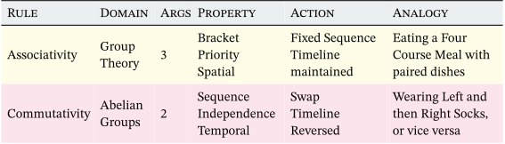
Associativity requires three elements. Commutativity is confined to two.
Associativity: The sequence cannot be changed
Let \(a\), \(b\), and \(c\) be arbitrary elements of a Group with a binary action \(\ast\). Because our mathematical operators are binary, they can only consume two inputs at a time. We cannot compute \(a \ast b \ast c\) in a single stroke; we must fuse them first in pairs. If we are presented with a chain of operations like \(a \ast b \ast c\), how do we evaluate this expression so that we get consistent results? The Associative Law guides us. It says \[(a \ast b) \ast c = a \ast (b \ast c) = a \ast b \ast c.\qquad{(5)}\] The brackets here have the same sense as in BODMAS—temporal priority. What we memorized in primary or elementary school during our mathematical innocence is the same result we get by applying Equation 5.
Note that the sequence is linear, not cyclic. The associative law does not deal with \(c \ast a \ast b\) at all. This is an important point to beware.
If you cast your eyes at Equation 5 and scan it from left to right, you will realize that the relative positions of \(a\), \(b\), and \(c\) are preserved all the way, intervening brackets notwithstanding.28
What has remained unchanged all along? The relative positions of \(a\), \(b\), and \(c\) have remained unchanged. Yes, they may have been bracketed and paired differently, but the relative positions of the three operands have not been altered. Nowhere do we see a sequence like \(a \ast c \ast b\). This preservation of the sequence is the sacred duty of Associativity.
To repeat, the brackets simply denote what I call “bracket priority” along the lines of BODMAS. It denotes which actions are performed first. You could also think of the brackets as “packaging” pairs of operands. The associative law demands that the relative order of the terms in the sequence \(a\), \(b\), \(c\) cannot be altered when we evaluate an expression obeying the associative law. Which pair we evaluate first does not alter the results.
Two other points should be borne in mind:
The associative law applies to three arguments or operands. Its primary purpose is to safeguard consistent evaluation when a binary operator has to deal with a succession of three chained operands.
According to our everyday perception, associativity feels more space-like than time-like. If you think of the operands as pickets in a fence, “packaging” terms or grouping them by “bracket priority” does not move the pickets. But the sequence itself may be viewed as a time-line. In this sense, associativity does not disturb the sequence, whether it is viewed through the lens of space or of time.
The confusion between associativity and commutativity arises because we learned the rules of arithmetic with numbers and transferred them later to algebra. But numbers are not ideal objects from which to learn lessons about the laws of abstract algebra.
This is because addition and multiplication are not only associative, they are also commutative. More about that in the next section.
Finally, an example to round off our discussion. Consider a three-step manufacturing process:
(B) Spin the yarn, and
(C) Knit the sweater.
The physical timeline is strictly \(A \to B \to C\). Any modification to this sequence will yield nonsense. The brackets below merely dictate how we organize our factories:
\((A \ast B) \ast C\): Factory 1 shears the sheep and spins the yarn, then ships it to Factory 2 to be knitted.
\(A \ast (B \ast C)\): Factory 1 only shears the sheep, shipping the raw wool to Factory 2 which spins and knits it together.
The timeline never changed. The chronological sequence of the wool’s transformation is identical. The brackets do not alter the arrow of time; they simply indicate which two actions were fused together first.
Commutativity: Swapping the Timeline
Commutativity, written as \[a \ast b = b \ast a,\] is the dangerous luxury of sequence independence. It asks: “Can I swap the chronological order of two actions?” In our factory analogy, this would be the equivalent of trying to spin the yarn before shearing the sheep. Commutativity is not common in nature because it does not make sense. But when it does, commutativity can lend great power, because of its rarity.
Associativity requires three arguments and preserves the
sequence.
Commutativity requires only two arguments and reverses the sequence with a straight swap.
Notice the quintessential distinguishing factor: Commutativity only requires two arguments because it is fundamentally a swap. We only need two items to exchange their chronological positions.
Associativity requires three arguments because it is about a picket fence. To prove that a boundary can be shifted without breaking the timeline, you must have a “middleman” (the \(b\) in our equation) to demonstrate that it can fuse just as safely with the action before it as it can with the action after it.
Summary
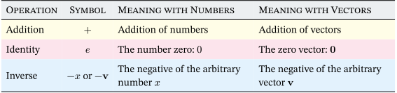
The table below summarizes what we have tried to clarify. Associativity preserves the sanctity of the sequence. Commutativity reverses the sequence with impunity.
Symmetry: The Overloaded Word
Mathematics occasionally suffers from a severe case of linguistic overloading. We recycle familiar words to mean entirely different things depending on the mathematical context. Perhaps no word is more abused in this way than symmetry. If you are feeling flummoxed by its multiple personalities, you are not alone.
To prevent confusion as we climb to the higher reaches of abstract algebra, we must unpack the distinct ways mathematics uses—and misuses—this word.
Symmetry as a mirror image
This is the symmetry of our childhood. It is the bilateral symmetry of a butterfly’s wings, or the reflection of a mountain in a still lake. In classical geometry, an object is symmetric if you can draw a line down its centre and fold it perfectly upon itself. It is a visual, static property of a shape.
Symmetry as a mutual connection
Before we even combine numbers, set theory introduces symmetry as a two-way street between elements. If we define a rule that links elements together—a relation \(R\)—we say the relationship is symmetric if \(aRb\) \(bRa\).
If Alice is a sibling of Bob, Bob is inevitably a sibling of Alice. (Contrast this with “is a parent of”, which is decidedly a one-way street). This mutual recognition is a cornerstone of an equivalence relation. Notice that unlike an algebraic operation, which combines two elements to create a third, a relation merely asks a true-or-false question: are these two things connected? If the connection always points both ways, the relation itself possesses symmetry.
The typographic illusion of symmetry: Commutativity
When we write \(a \ast b = b \ast a\), the equation itself looks symmetrical on the page. Because of this visual balance, commutativity is often colloquially—and mistakenly—called “symmetry of operation”. But this is a typographic illusion.
Commutativity is an internal combining of elements that never leaves the original space; it strictly maintains set closure. Conceptually, this is the sequence independence of the timeline. It guarantees that the chronological order of two events can be swapped without altering the final internal state. It is not true mathematical symmetry because it does not measure; it combines.
Symmetry as reversibility
This is the profound structural symmetry of Group Theory. It has nothing to do with mirror images and everything to do with actions. In a group, symmetry means unconditional reversibility, i.e., \(f \ast f^{-1} = e = f^{-1} \ast f\). Every action one takes has a guaranteed counter-action that will reliably restore the universe to its original state.
A Rubik’s cube possesses immense group symmetry because every twist can be mathematically undone—even though twisting the right face and then the top face is fiercely non-commutative.
But you might retort that \(f \ast f^{-1} = e = f^{-1} \ast f\) is an example of commutativity. And that is an entirely justified doubt to raise at this point.
An element commuting with its own inverse is a strict, exclusive relationship.29 They are perfectly matched opposites, designed to annihilate each other into the identity element \(e\) no matter which one goes first. Think of it like taking exactly one step forward and one step backward. You could equally well have taken one step backward and one step forward. The order does not matter; you end up exactly where you started. Any element and its inverse share this exclusive relationship.
Commutativity requires \(f \ast g = g \ast f\) for any pair of elements, \(f\) and \(g\). And that is not the case here.
An example of symmetry at two levels
Sometimes these different masks of symmetry align stunningly. Consider the natural exponential function \(e^x\) and the natural logarithm \(\ln(x)\). As explored previously in my blog The Exponential and Logarithmic Functions, they act algebraically as exact inverses—a bijection where one operation entirely undoes the other. Moreover, if we plot them on a graph, this algebraic reversibility manifests visually as a perfect mirror image reflected across the diagonal line \(y = x\). The algebraic symmetry of “undoing” transforms directly into the geometric symmetry of our childhood.
Symmetry as measurement
We met conjugate relational symmetry in the Inner Product Space, where \(\langle \mathbf{u}, \mathbf{v} \rangle = \overline{\langle \mathbf{v}, \mathbf{u} \rangle}\). Here, we are no longer combining elements to create a new one within the set; we are stepping outside the space entirely to evaluate a relationship.
The mathematical shadow \(\mathbf{u}\) casts on \(\mathbf{v}\) is precisely the complex conjugate of the shadow \(\mathbf{v}\) casts on \(\mathbf{u}\).
It is the guarantee that measurement is independent of perspective—the distance from your house to the tropical rain forest is exactly the same as the distance from the forest back to your house. Symmetry deliberately breaks closure to measure: the measurement is done in another set entirely.
The last word on symmetry is:
Symmetry is invariance under transformation.
Why Associativity is the Bedrock
Now that we have untangled the four faces of symmetry, a startling realization emerges: the ability to casually swap the sequence of events—commutativity—is not a fundamental law of Nature. It is a fragile luxury that only exists in highly specialized spaces.
This begs a profound question: if we strip mathematics down to its foundational pillars, past the numbers and the equations, what actually holds the edifice together?
We are left with functions. A function is simply a verb—an action that transforms an input into an output. When we chain these actions together so that the output of the first becomes the input of the second, we are performing function composition.
Because function composition is the fundamental driver of all mathematics, its inherent properties dictate the laws of the mathematical universe. And the single, inescapable property of function composition is associativity.
Associativity is one of the deepest structural principles underlying composition. It guarantees that when we chain operations together, the sequence of execution does not destroy the integrity of the final result. It is the invisible glue that holds sequential logic together.
Imagine a meal. There is an expression called “from soup to nuts” describing the sequence of dishes. We progress from soup to salad through the main course to dessert and nuts. This sequence is sacrosanct. But we might be served soup along with the salad. Bracketing soup with salad does not offend the correct sequence of courses. Mind you it is (soup + salad) not (salad + soup).
Commutativity, however, attempts to swap any two courses anywhere in the sequence. Imagine starting with dessert and ending with soup. That would upset your expectations, your palate, and perhaps even your stomach!
This is exactly why matrix multiplication is associative but famously non-commutative. A matrix is not just a grid of numbers; it is the algebra of a linear transformation—a function. Matrix multiplication is literally function composition. If matrix \(A\) transforms a 2D plane into 3D space, and matrix \(B\) transforms 3D space into 5D space, they are strictly ordered. The output of \(A\) (3D) matches the input of \(B\) (3D). They are, to use the apt phrase, conformable in that specific sequence.
If you attempt to commute them and apply \(B\) first, you are trying to feed a 2D plane into an input expecting 3D space. The interfaces do not fit. The operation is undefined. Even when the matrices are perfectly square and the links do fit, swapping the order of actions—like rotating a shape \(90^∘\) and then reflecting it in a mirror, versus reflecting it first and then rotating it—produces an entirely different final state.
Associativity is the structural bedrock of chaining operations
together.
Commutativity is a fragile luxury.
An overview of Abstract Algebra
Just as a dying man says the most important things first, to maximize information transfer, we have, until now, concentrated upon the most widely used algebraic structures. It is now time to do a top to toe survey and draw charcoal thumbnail sketches of much of abstract algebra. The treatment will be condensed and generously illustrated with tables and diagrams.
Exorcising the ghost of jargon
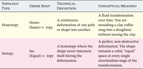
Incomprehension arising from not knowing the jargon is most off-putting. Just think of a hospital emergency room and the buzz of medical terms used there routinely and you will experience the precise feeling that assails the newcomer to abstract algebra. To help overcome this, Figure 12 is a concise summary of terms, that is accessible to the layperson without losing mathematical precision.
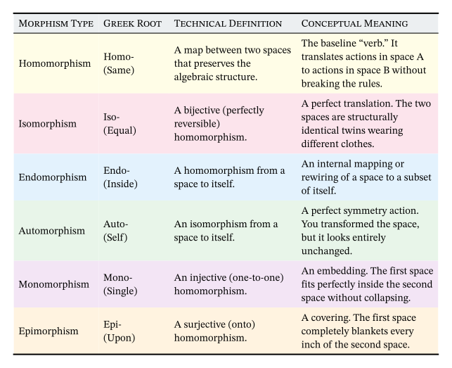
If algebra is the study of structure/shape—and its actions are denoted by the suffix morphism which means “having a particular form or shape”—topology is the study of place/space and the Greek suffix topy denotes place or position. Words ending in “topy” are encountered when mathematical objects are deformed over time.
The Ascent of Mount Abstract Algebra
If we start with absolute, formless anarchy we may slowly forge it into a rigid geometric and algebraic object by enforcing one new rule at a time. We could either ascend a hierarchy of nested structures, or we could descend into a set of Russian Dolls, where each deeper structure inherits all the rules of the larger shells that contain it, while adding a strict new constraint of its own. Whichever the metaphor, we are on a journey of exploration, which I have called the “Ascent of Mount Abstract Algebra”.
In each case we try to answer four questions about the abstract algebraic structure:
Name \(\to\) Etymology
Why \(\to\) Need
What \(\to\) Characteristics
How \(\to\) Examples
We first examine the names of the structures themselves.30 Mathematical nomenclature often seems deliberately opaque, but looking at the etymology of these words reveals exactly how the pioneers viewed these structures as they were discovering them. We then briefly review why these structures came to be, followed by their characteristics, and some examples of the structures.
Magma: The Formless Paste
Coined by the influential 20th-century French mathematical collective Nicolas Bourbaki. It derives from the Greek magma (μαγμα), meaning a thick paste or kneaded dough. Bourbaki used it metaphorically to describe a mathematical structure that is fluid, formless, and primitive—a raw “molten” set with one operation, before cooling and crystallizing into the more rigid rules higher up the mountain.
We require an absolute base camp—the simplest possible algebraic structure. If you throw away every single rule of mathematics except the guarantee that an action actually produces a valid result without breaking the system, what is left? A Magma.
It is a set equipped with a single binary operation that satisfies exactly one rule: Closure. If you take any two elements \(a\) and \(b\) in the set, \(a \ast b\) must produce an answer that also lives inside the set. Nothing else is demanded. A particular magma may happen to be associative, or have an identity, or have inverses—for every group is a magma, after all—but the definition does not promise any of these.
In the framework of our Matryoshka dolls, the Magma is the largest, outermost shell. While highly disciplined structures like Groups technically live inside Magmas—just as every square is a rectangle—a “strict” Magma is a structure that possesses only closure. Because it fails all further rules, it cannot fit into any of the smaller, deeper dolls.
Consider subtraction on the integers (\(a - b\)). The result is always an integer, so it is closed and is a Magma. But \((5 - 3) - 2 \neq 5 - (3 - 2)\); so this particular magma is not associative: the timeline is broken.
Another everyday example is taking the average of two numbers. The result is always a valid number, guaranteeing closure. But the grouping changes the final answer: averaging \(2\) and \(6\) gives \(4\), and averaging that with \(10\) yields \(7\). However, grouping \(6\) and \(10\) first gives \(8\), and averaging that with \(2\) yields \(5\). It is a strict Magma, but nothing more.
Semigroup: The Half-Baked Group
A straightforward linguistic hybrid of the Latin semi- (half) and “group”. It possesses exactly half of the strict rules of a full group: it has closure and associativity, but lacks an identity element and inverses.
A Magma is too chaotic to be of much use. We need the arrow of time to be respected so we can build reliable, logical chains of cause and effect. We need to be able to safely drop the parentheses in a long string of operations without ambiguity.
A Semigroup is a Magma plus the rule of Associativity. Now, \((a \ast b) \ast c = a \ast (b \ast c)\). The chronological sequence of actions is preserved, no matter how the mathematician packages or groups them.
Let our set be “Strings of text”. If the operation is “concatenate”—conjoining words together—then (“head” + “light”) + “bulb” is the same as “head” + (“light” + “bulb”). It always yields “headlightbulb”.
Monoid: The Realm of the “One”
From the Greek monos (single or alone) and the suffix -oid (resembling or shape). In abstract algebra, the “single” thing it refers to is the identity element—the solitary, immovable anchor that a semigroup lacks.
In early mathematics, the identity element was almost universally referred to as “the unit” or “the one”, since \(1\) is the identity for multiplication, the default operation of early study. Therefore, a Monoid is literally “a structure characterized by having a ‘One’.” The moment a Semigroup gives birth to an identity element, it is christened a Monoid in honour of that very element.
We need the ability to “do nothing.” If we are building a system of actions, we must have a baseline state of rest. In computer programming, if we want to loop through a list and accumulate a result, we need a starting value that does not inadvertently alter the total. In a clinical drug trial, it is the placebo—an administered action that leaves the body perfectly unchanged. In a gearshift motor car, it is the neutral gear.
A Monoid is a Semigroup that has an added Identity Element, often denoted as \(e\). There must exist an element \(e\) where \(a \ast e = a\) and \(e \ast a = a\).
Returning to strings of text, the identity is the empty string
"". The string (“hello” + "") = “hello”. In
standard arithmetic, the whole numbers \(\{0,
1, 2, 3...\}\) form a Monoid under addition, where the identity
element is \(0\). It is not yet a group
because there are no negative numbers to reverse the addition.
Group: The Cluster
Coined by the tragic mathematical genius Évariste Galois around 1830. He used the French word groupe (from the Italian gruppo, meaning a knot or cluster) simply to describe a collection of permutations that “grouped together” under composition to act as a closed, unified system.
He noticed that certain collections of permutations always chained together to produce another permutation within that same collection. They clustered together, entirely closed off from the rest of the universe. He casually called this cluster a “group,” and the mundane name stuck to the most profound symmetry concept in the mathematical cosmos.
In a Group, we need the ability to undo an action. Without reversibility, we can only move forward, eventually getting trapped in a state we cannot escape. True mathematical symmetry requires an undo button that always works.
A Group is a Monoid plus Inverse Elements. For every element \(a\), there exists an element \(a^{-1}\) such that \(a \ast a^{-1} = e\), and \(a^{-1} \ast a = e\). Every action has a guaranteed counter-action that restores the universe to its original state.
All integers (\(\mathbb{Z}\)) under addition form a Group. The inverse of \(5\) is \(-5\), because \(5 + (-5) = 0\). Geometrically, the Rubik’s Cube is a Group. Every twist is an action, and no matter how scrambled the cube becomes, there is a sequence of inverse actions that will perfectly restore it to a solved state. In a motorcar, the reverse gear performs this function.
Abelian Group: The Commuting Cluster
This group is named after Niels Henrik Abel, and we have touched upon its etymology previously in the section Groups and Abelian Groups in this blog.
Why was this special name required, rather than just making commutativity a standard group rule? Because the most vital, foundational structures in mathematics—such as the symmetries of polynomials, rotations in 3D space, and matrix operations—are stubbornly non-commutative. If mathematicians had mandated commutativity, Group Theory would be entirely incapable of describing the physical and algebraic universe. Commutativity was recognized as a highly specific property, not a universal law. So, a special type of group—one that strictly obeys this sequence independence—was identified and brought into the fold under Abel’s name.
We occasionally require sequence independence. To navigate physical geometry or do basic accounting, we need a space where the chronological order of operations can be safely ignored.
An Abelian Group is a Group plus Commutativity. Now, \(a \ast b = b \ast a\). Vector addition is commutative. If you walk 3 blocks East and 4 blocks North, you arrive at the same destination as walking 4 blocks North and 3 blocks East. The geometric grid requires commutativity to remain stable.
Ring: The Number Ring
The term is generally traced to David Hilbert’s use of Zahlring or “number ring”. He was studying sets of algebraic integers that “circled back” on themselves when subjected to specific operations. The term was later formalized by Emmy Noether, who stripped away the specific numbers and defined the abstract axioms we use today.
A Group only gives us one tool, like addition. To build true arithmetic, we need two interacting tools: addition and multiplication. We need a system where we can scale and stretch elements, not just slide them around.
A Ring is an Abelian Group, with addition, that introduces a second operation, multiplication. This new multiplication must be a Monoid—it is associative and has an identity element, \(1\)—and crucially, it must distribute multiplication over addition: \(a \times (b + c) = (a \times b) + (a \times c)\).31
Square matrices can be added (as an Abelian Group), and we can multiply them. They are associative, but notoriously non-commutative. The combination of these two operations makes the set of square matrices a Ring.
Commutative Ring: The Harmonious Ring
Matrix multiplication is non-commutative. For standard numbers and polynomials, we want multiplication to be sequence-independent as well. A Commutative Ring is where the second operation, multiplication, is now Commutative: \(a \times b = b \times a\).
Examples are the integers \(\mathbb{Z}\) under ordinary addition and multiplication, and the integers modulo \(6\): the “clock-face” numbers \(\{0, 1, 2, 3, 4, 5\}\), where we add and multiply as usual and then keep only the remainder on division by \(6\). In both we can add, subtract, and multiply in any order—e.g., \(2 \times 4 = 4 \times 2\)—and multiplication distributes perfectly over addition. But neither is a Field, because we cannot always divide: in \(\mathbb{Z}\), for instance, \(2 \div 4\) is not an integer.
Integral Domain: No Zero Divisors
This name is a direct homage to the integers \(\mathbb{Z}\). An Integral Domain is a Commutative Ring (with \(1 \neq 0\)) that perfectly mimics the multiplicative reliability of the integers—specifically, the guarantee that you cannot multiply two non-zero numbers and magically get zero.
We need to prevent mathematical anomalies where multiplying two distinct “things” mysteriously yields “nothing.” We need to ensure that if the final product is zero, one of our starting components was definitely zero. A Commutative Ring that eliminates Zero Divisors is an Integral Domain. If \(a \times b = 0\), then either \(a = 0\) or \(b = 0\).
All integers (\(\mathbb{Z}\)) under addition and multiplication form an integral domain. Contrast this with the integers modulo \(6\), where \(2 \times 3 = 6\), which leaves a remainder of \(0\), although neither \(2\) nor \(3\) is zero. This is a commutative ring in which two non-zero elements multiply to give zero. It is precisely this kind of anomaly that Integral Domains rule out.
Matrices show the same phenomenon of zero divisors, even more strikingly. Here is a classic example of two non-zero matrices multiplying to yield the zero matrix. Let \[A = \begin{bmatrix}1 & 0 \\ 0 & 0\end{bmatrix} \text{ and }B = \begin{bmatrix}0 & 0 \\ 0 & 1\end{bmatrix}.\] Although neither \(A\) nor \(B\) is zero, their product \(AB\) is zero: \[AB = \begin{bmatrix}0 & 0 \\ 0 & 0\end{bmatrix}.\] Because these “zero divisors” exist, the set of square matrices is not an Integral Domain. (It fails twice over: matrix multiplication is also notoriously non-commutative.)
Ideal: The Mathematical Black Hole
Coined by Ernst Kummer in the 1840s when he invented “ideal numbers” to fix the failure of unique prime factorization in certain complex number systems. Emmy Noether later abstracted this concept into the algebraic structures we use today.
In a Ring, we can add, subtract, and multiply elements. But often, we want to look at “multiples” of a specific element or subset—much like how all even numbers form a self-contained subset of the integers. We need a systematic way to collapse or “swallow” parts of a ring to form smaller, simpler quotient structures, just as modulo arithmetic simplifies numbers.
An Ideal is a special subset of a Ring that absorbs multiplication from the outside. While a subring must contain its own multiplicative identity and be a ring in its own right, an Ideal is much greedier: if you take any element inside the Ideal and multiply it by any arbitrary element residing anywhere in the parent Ring, the product is yanked back inside the Ideal. In modern algebra, an Ideal acts like a mathematical “black hole” within a Ring.
Consider the ring of integers \(\mathbb{Z}\). The set of all even integers (multiples of \(2\), denoted \(2\mathbb{Z}\)) forms an Ideal. If you take any even number (say, \(4\)) and multiply it by any integer at all (say, \(5\)), you get \(20\), which is still even and lives inside \(2\mathbb{Z}\). Another example is the set of polynomials divisible by \(x\) in the ring of polynomials: multiplying any multiple of \(x\) by any other polynomial always yields another multiple of \(x\).
Field: The Sovereign Body
The English term field was coined by the American mathematician E H Moore in 1893. He was translating the concept from the German Körper, meaning “body”, which Richard Dedekind had introduced in 1871. Moore chose “field” to evoke the idea of a self-contained plot of land where one could wander without ever stepping outside its boundaries. It was a domain of numbers where the four arithmetic operations—addition, subtraction, multiplication, and division—were closed.
We have reached the summit of arithmetic. We need absolute freedom of motion. We must be able to infinitely scale up, and infinitely scale down. We need division.
A Field is an Integral Domain where every non-zero element has a Multiplicative Inverse32. You can add, subtract, multiply, and divide flawlessly.
This explains the “division by zero is prohibited” rule.33 Without it, we cannot find polynomial roots.
The Rational numbers (\(\mathbb{Q}\)), Real numbers (\(\mathbb{R}\)), and Complex numbers (\(\mathbb{C}\)) are the comprehensively equipped arenas where standard algebra and calculus are born.
Vector Space: The Geometric Grid
From the Latin vector, meaning “a carrier” or “one who conveys”, from vehere, to carry.34 Sir William Rowan Hamilton introduced the term in the 1840s to describe the geometric part of a quaternion that literally “carries” a point from one location to another in space.
While a Field provides perfect numbers for arithmetic, it lacks geometry. We need a way to describe physical space—to model directions, forces, velocities, and multi-dimensional grids. We need a structure that marries geometric directions (vectors) with arithmetic scaling (scalars from a Field).
A Vector Space is a hybrid structure built from two distinct sets. The “vectors” form an Abelian Group under addition (you can add geometric arrows together). But crucially, they are subject to “scalar multiplication” by elements from an external Field. The rules dictate how the Field stretches or shrinks the vectors flawlessly without breaking the grid.
The classic 2D Cartesian plane (\(\mathbb{R}^2\)) and 3D space (\(\mathbb{R}^3\)) are vector spaces. The vectors are coordinates like \((x,y)\), and the Field providing the scalars is the Real numbers (\(\mathbb{R}\)).
“Minor” Algebraic Structures
The structures outlined so far from Magma to Field form the primary backbone of abstract algebra. However, there are a few “minor” or specialized structures that branch off this main path. We will briefly introduce them here for the sake of completeness.
Lattice: The Geometry of Order
Coined in the 1930s and popularized by Garrett Birkhoff. The name was chosen purely for its visual geometry: when you draw the hierarchical relationships—the Hasse diagrams—of these structures, the crossing lines visually resemble a wooden garden lattice or trellis..
Not every mathematical structure is about arithmetic or combination, like adding or multiplying. Sometimes we need to study hierarchies, ranking, and logical constraints—how elements relate to each other in terms of “higher than” or “lower than”.
A Lattice is a partially ordered set in which every two elements have a unique greatest lower bound (meet) and least upper bound (join). It trades arithmetic operations for a geometry of order. The same idea is encountered in much of mathematics under different names, and Figure 14 is a summary of these new terms.
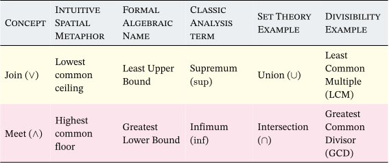
Think of finding the least common multiple or greatest common divisor in a divisibility lattice. Propositional logic and set inclusion also form natural lattices, as illustrated in Figure 14.
Module: The Ring-Scaled Grid
From the Latin modulus, meaning “a small measure” or “a standard” (sharing a root with modular arithmetic and architectural modules). Richard Dedekind introduced it in the context of algebraic integers because modules act as a standard frame of reference for measuring properties within rings.
Vector spaces require scalars to come from a Field—meaning we must always be able to divide by any non-zero scalar. But what happens when our scaling numbers come from a structure where division is impossible, such as the integers or polynomial rings? We need a more flexible grid that relaxes this strict requirement.
A Module is what you get when you weaken a Vector Space: it is a grid scaled by a Ring instead of a Field. Because Rings lack division, Modules lose many rigid properties, such as the guaranteed existence of a basis. Most strikingly, Modules can possess torsion—a phenomenon where multiplying a non-zero element by a non-zero scalar mysteriously collapses the result down to zero.
Every Abelian group is automatically a module over the ring of integers \(\mathbb{Z}\), where scaling an element by an integer simply means repeated addition (or subtraction). Ordinary vector spaces are just the special case where the scaling ring happens to be a fully equipped field.
Algebra (over a Field): The Multiplicative Hybrid
From the Arabic al-jabr (“reunion of broken parts”), historically applied to the balancing and solving of equations. In modern abstract algebra, the word was repurposed to denote a vector space equipped with a well-behaved internal multiplication.
In a standard Vector Space, vectors can be added to each other and scaled by numbers from a field, but they cannot be multiplied together. To model physical and geometric phenomena where vectors interact directly through multiplication while respecting the underlying grid, we need an even richer structure.
An Algebra over a Field is the ultimate structural hybrid. It acts simultaneously as a Vector Space and a Ring (or multiplicative system). It is a Vector Space where we are also allowed to multiply the vectors themselves together in a way that perfectly respects the grid, satisfying distributive laws with the scalars.
Ordinary Euclidean space equipped with the vector cross product in 3D physics forms a non-associative algebra. Another premier example is Hamilton’s quaternions (\(\mathbb{H}\)); operating as a 4-dimensional vector space over the real numbers, they allow full multiplication and division, making them a division algebra, even though their internal multiplication is famously non-commutative.
The complete picture
I will round off this brief survey of the major algebraic structures with two diagrams
- Figure 15. This may be viewed as an “architectural plan view” showing nested Russian dolls or Venn diagram rectangles of the principal structures of Abstract Algebra. It demonstrates how successive structures are encased within stricter rules.
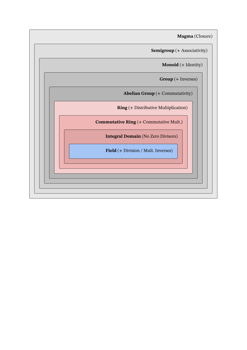
- Figure 16. This may be viewed as the “architectural elevation view” of the same monument of abstract algebra showing how mathematics is constructed from the ground up, resting on the foundation of Magma.
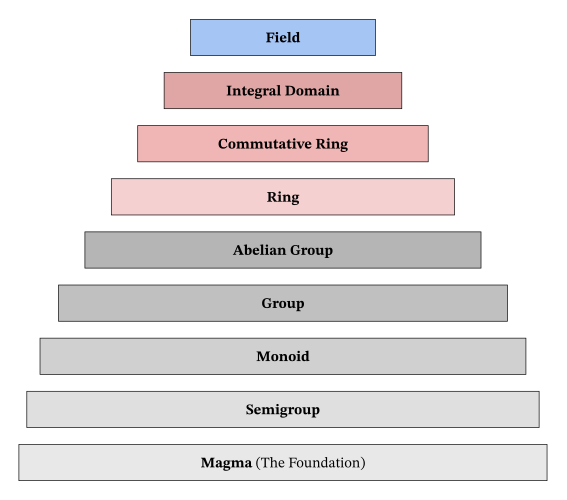
“Abstract. Simplify. Generalize.” in reverse
In his book The Art of UNIX Programming [5], the open-source software pioneer Eric S Raymond wrote a three-word mantra: “Abstract. Simplify. Generalize.” The section in which this formula occurs is interestingly called “Compactness and Orthogonality”. It shows how close Computer Science is to its parental roots in Mathematics.
Historically, the pioneers of mathematics ironically repeated Raymond’s mantra in reverse while developing abstract algebra. They began by generalizing a specific mathematical pattern, like the symmetries of polynomial roots, or the addition of physical force vectors. Once the pattern was identified, they simplified it by ruthlessly paring away everything except a frugal list of core axioms. Finally, they abstracted those axioms completely away from their original physical context, creating the pure, formless spaces we have just explored. Abstract Algebra is the art of starting with the concrete and refining it until only the irreducible structural truth remains.
The Distilled Essence: Abstract Ideas in Their Purest Form
As we step back from our survey of the algebraic landscape, it is worth reflecting on what this ascent actually leaves in our hands. If we strip away the thickets of notation, the Greek symbols, and the specific number systems, we find that abstract algebra is not merely a collection of assorted truths, it is also a distillation of universal cognitive tools.
In fact, if we take the rigid axiomatic hierarchy we have just climbed and project it onto a different set of conceptual “basis vectors”, a profoundly different vocabulary emerges. We see pure, unadorned ideas that govern not just algebra, but all of quantitative and logical thought:
Order: The architecture of precedence. From the simple comparative ranking of elements to the intricate geometry of lattices, order allows us to establish hierarchy and structural flow without ever needing numbers to measure size.
Bounds: The ceilings and floors. These are the suprema and infima that establish absolute limits. Bounds prevent mathematical spaces from drifting into an amorphous haze by anchoring them to definitive extremes.
Symmetry: The structural harmony of form. Whether it is the static mirror image of classical geometry or the dynamic, reversible choreography of group actions, symmetry provides the overarching framework for how a system balances itself.
Invariance: The steadfast core. If symmetry is the transformation, invariance is what survives the storm. It is the underlying truth—a quantity, relation, or property—that remains utterly unchanged while the universe around it is rotated, reflected, or permuted.
Inclusion and Exclusion: The logic of boundaries. This governs what is permitted inside a system, which sub-structures (like ideals) act as mathematical black holes to absorb outside elements, and what is formally banished across the frontier.
Action and Scaling: The arithmetic engines. These are the groups, rings, and fields that provide the formal machinery for magnitude and operational closure. They define the precise hierarchy of capabilities, moving from reversible actions to distributive scaling, and ultimately to absolute arithmetic freedom.
These abstract threads do not just organise mathematics; they provide the conceptual vocabulary through which we model reality itself.
First steps to Galois Theory
On the night of May 29, 1832, a twenty-year-old Évariste Galois sat at his desk, feverishly writing a mathematical testament to his friend Auguste Chevalier. He was due to fight a pistol duel at dawn—a duel he rightly suspected would end his life the next day. In the margins of his frantic notes, he scribbled, “I have no time.” Yet, in those desperate final hours, he outlined an epiphany that would permanently alter the landscape of mathematics.
For nearly three centuries, the greatest minds in Europe had been searching for a universal formula to solve the quintic—a polynomial equation of the fifth degree. They were looking for a mathematical oil mill, similar to the quadratic formula, where one could press the coefficients through a series of additions, subtractions, multiplications, divisions, and root extractions to output the oil of the roots. By the early nineteenth century, Paolo Ruffini and Niels Henrik Abel had proved the unthinkable: no such universal formula exists for the general quintic. That left a deeper question: why do some equations yield to such formulas and others do not?
Galois realized they were asking the wrong question.
Instead of trying to calculate the exact numerical values of the roots (the nouns), Galois decided to study the symmetries of the roots (the verbs).
We can glimpse this genius using high school algebra. Consider a standard quadratic equation with two roots, \(\alpha\) and \(\beta\). Even if we do not know the exact numerical values of \(\alpha\) and \(\beta\), we know from the coefficients of the equation that their sum \((\alpha + \beta)\) and their product \((\alpha\beta)\) are fixed numbers directly determined by the equation’s coefficients.35
Notice the inherent symmetry. Swapping \(\alpha\) and \(\beta\), the sum becomes \(\beta + \alpha\) and the product becomes \(\beta\alpha\). Because addition and multiplication are commutative, the results are completely unchanged. The underlying algebraic structure is immune to this swap.
Galois scaled up this intuition to polynomials of any degree. He asked a profound question: “If I shuffle the unknown roots of an equation around in every conceivable way, which specific shuffles leave the underlying arithmetic relationships perfectly intact?”
These valid shuffles are actions, and they can be chained together via composition. They include a “do nothing” state, or identity. Moreover, every shuffle can be perfectly undone through inverses. In that flash of insight, Galois realized that the valid symmetries of the roots formed a rigid, closed architecture—a Group.
If this “Galois Group” could be broken down into simple, commutative building blocks, or Abelian groups, the polynomial could be solved with a formula. But if the Group was too hopelessly entangled—as it is for the general quintic equation—no formula could ever exist. The geometry of the symmetries forbade it.
Galois used Group Theory to measure the structural limits of a Field. But before we can study how these roots dance with one another, we must first mathematically guarantee that the stage exists, and that the roots actually show up to perform. That absolute guarantee is known as the Fundamental Theorem of Algebra, and it will be the starting point for our next mathematical expedition.
Suggestions for Further Reading
I trust that this blog has removed any unease you might have had toward Abstract Algebra. By now, you would hopefully have an overview of the structures of Abstract Algebra, their rationale, characteristics, and applications. But mathematics is all about doing—to ground the ethereal constructs—either by proving theorems, or by applying them in practice. With that in mind, I have four expositions to suggest for further reading, listed by author.
B A Sethuraman’s A Gentle Introduction To Abstract Algebra [6] is a rare textbook on several counts. It is unhurried and conversational in its approach, taking the time to explain the why behind the definitions, making it an ideal companion for the independent scholar. It is colour-coded, making it easy to navigate through examples, questions, and exercises. It is freely available online, ensuring that the beauty of mathematics remains accessible to the curious layperson. Given his pedagogical style, I would also recommend Professor Sethuraman’s Proofs and Ideas for the aspiring mathematician who is just starting out.
Lara Alcock has written a series of books to help students orientate themselves to study mathematics at university. Among these is her aptly named book How To Think About Abstract Algebra [7]. It eases the student gradually into the subject, moving from the known to the unknown. It is a good starting point to learn abstract algebra formally.
Thomas Q Sibley has written several books, just like Alcock and Sethuraman. Given the contemporary milieu for specialization, it is highly unusual for a university professor to write books on both Geometry and Abstract Algebra. If he does so, it not only signifies subject mastery but also a gift for exposition. His Thinking Algebraically: An Introduction to Abstract Algebra [8] might be more demanding than the first two, but it is well-written, and lavishly peppered with examples.
Derek J S Robinson’s Abstract Algebra: An Introduction with Applications [9] is my fourth recommendation. It is the closest to a traditional mathematics textbook. The writing is clear, uncluttered, and brisk. It would be a go-to reference if you ever get stuck.
Over and above these, in the course of writing this blog, I have come across two texts that I can only describe as “mind expanders.” I list them below:
Jürgen Jost’s Mathematical Concepts [10] provides a panoramic survey of mathematics that is surprisingly accessible but also predictably deep. If ever you want to probe further into that dark forest hidden behind wooden doors, this book could be your guide. The trick in reading it is to read it only insofar as you get the drift. Going any deeper could lead to scholarly fatigue.
George Bergman’s An Invitation to General Algebra and Universal Constructions [11] universalizes algebra and is a good follow-on to the above-recommended texts. It is a surprisingly reader-friendly text even though it delves into the unexposed depths of contemporary algebra.
Do look them up if you can.
Acknowledgements
I owe a debt of gratitude to George F Simmons, whose classic text Introduction to Topology and Modern Analysis [12] pioneered the use of nested Venn diagrams to demystify the relationships between mathematical spaces. His pedagogical clarity inspired the visual approach used for the Magma-to-Field hierarchy in this blog—an example that I am surprised and saddened to see so few others emulate.
The title of this blog was inspired by the title of Paul Hewitt’s book Conceptual Physics [13] which is now in its richly deserved thirteenth edition.
This blog was written with a collaborator whose face I have not seen: Google Gemini. Perhaps the greatest benefit from this cooperation has been the rapidity and specificity of answers to questions. The to-and-fro conversation made learning both fast-moving and enjoyable. To Google Gemini my grateful thanks. As always the blog will be refereed by at least two other AIs before being published.
Feedback
Please email me your comments and corrections.
A PDF version of this article is available for download here:
References
A slog is a long blog.↩︎
Category Theory calls the nouns Objects and the verbs Morphisms. This is simpler but has its drawbacks, and is therefore not used here.↩︎
Semigroups have the foundational property of associativity (sequence preservation), and Monoids possess, in addition, the identity element (for the “do nothing” operation). These ideas will become clear later on.↩︎
The number \(i\) and the angle \(90°\) are called generators of \(C_4\) as the entire group may be generated by repeated application of the generator.↩︎
The use of logarithms is an example where a difficult multiplication problem is transformed isomorphically into an easier addition problem, and the result transformed back into the original domain to yield a result.↩︎
The formal language of “objects” (sets or algebraic structures) and “morphisms” (structure-preserving maps between them) originates from Category Theory, providing a unified vocabulary across mathematics.↩︎
Every isomorphism is fundamentally a homomorphism (a structure-preserving map) that also happens to be a perfect, reversible, one-to-one match between two sets.↩︎
See Groups and Abelian Groups later in this blog.↩︎
They are a large family but how they became so large is a story for another blog.↩︎
This axiom is vital because it ensures compatibility between geometric scaling in the vector space and algebraic scaling by scalar multiplication.↩︎
Closure is understood, and commutativity is tacit in the very adjective “Abelian”. They are therefore not highlighted here.↩︎
Conditions apply in all cases, but the facts are these.↩︎
“The Nothing That Is” is the title of the popular mathematics book written by Robert Kaplan and illustrated by Elen Kaplan. It is recommended reading for the interested layperson.↩︎
This absolute structural minimum should not be confused with the kernel of a group homomorphism or the nullspace of a linear transformation. Those are the collection of all elements in a domain that a specific function maps into the identity or zero vector of the target space.↩︎
These structures are named and explained later in this blog.↩︎
The various structures are named and discussed later in this blog.↩︎
Although mathematicians like Lagrange and Cauchy laid crucial groundwork, the formal structure of Groups was born from the tormented mind of Galois.↩︎
If you do not believe me, ask yourself whether you can brush your teeth and then wake up, or if you can eat your food and then cook it, or if you can scramble your egg and then break it. Nature and life are mostly non-commutative, and this is the tyranny imposed by time.↩︎
Note that while associativity requires a sequence of three arguments for its definition, commutativity requires only two.↩︎
See my blog Varieties of Multiplication if you new to this concept.↩︎
The complex conjugate is usually denoted as shown. Variants include a shorter bar over the \(z\) like \(\bar{z}\) or an asterisk superscript like \(z^{*}\).↩︎
Those of you who are familiar with programming will recognize this as the difference between an interface (which operations must exist, and which rules they must obey) and an implementation (the code that actually does the work).↩︎
This is called Hermitian symmetry—the real part exhibits even symmetry while the imaginary part exhibits odd symmetry.↩︎
In my blog on Varieties of Multiplication I have touched upon orthogonality. If you have studied Mechanics in high school, you will be familiar with the idea of the component of a vector in a particular direction. In the quoted blog, I have stated that “a force vector \(\mathbf{F}\) has no effect perpendicular to the direction in which it acts, and this is because its component or projection in that direction is \(\|\mathbf{F}\|\cos 90^∘ = 0\).”↩︎
Again, see my earlier blog Varieties of Multiplication.↩︎
Imagine Macbeth or Hamlet being enacted under these rules. Confusion will reign. This is why mathematics seems so daunting to so many.↩︎
Technically, these bracket pairs are called parentheses, but we call them brackets to retain a connection to the BODMAS mnemonic.↩︎
Like an electron and a positron.↩︎
This is the “getting to know you” party the night before the conference opens!↩︎
Some authors define a ring without requiring a multiplicative identity \(1\). We include it because our subsequent ascent to Integral Domains and Fields depends upon it.↩︎
In a Field, \(1 \neq 0\). Otherwise the one-element ring \(\{0\}\) would erroneously qualify as a Field.↩︎
See a previous blog that asks “why is division by zero disallowed?”.↩︎
Think vehicle.↩︎
See Completing the square and the quadratic formula for an explanation.↩︎